Python Modules – Layer and scan path calculations
Slice geometry, compare hatch paths and correctly interpret additive-manufacturing results.
No chapter found. Try another search term.
Chapter 01What you calculate with the Python package
The currently configured Python package contains python-additive, the “Additive Manufacturing – Layer Hatch” module. It cuts an uploaded triangle mesh and generates contour and hatch paths within that two-dimensional slice. You can change slice position, angle, spacing and selected process parameters, then examine the effects on path count, length and reported scan time.
This handbook addresses module users. Operating it does not require editing Python files. Developing new Python modules is a separate workflow; each new module needs its own engineering review and instructions. This package does not establish an additional automatically available collection of arbitrary Python calculations.
Interpreting the results
- Slice area describes the selected plane within the mesh, not the surface area or volume of the complete part.
- In the inspected source, the result path length sums hatch segments only. Additional contour paths appear in the visualization.
- The result scan time is hatch length divided by hatch speed. It is not total layer or build time.
- The coloured risk view is a simplified path-based assessment model. It replaces neither a validated thermal process simulation nor approval of machine parameters.
The teaching case uses a purpose-created 20 × 12 × 4 mm block. The unchanged calculation source was executed against it in an isolated Python environment. Values and path plots are actual results of that source execution; Web upload and a complete browser calculation were not executed.
Back to top ↑Chapter 02Opening the module and understanding the workspace
Open the module browser and search for python-additive or the displayed additive-manufacturing name. Whether it appears in your installation depends on its installed Python modules and runtime. The identifier is established by the local Python module descriptor; it is absent from the general legacy mask catalogue and should not be replaced there with an invented alias.
Three connected areas
- Mesh file: The upload area accepts an STL or OBJ file. After loading, it shows the filename and detected geometric bounds.
- Parameters: Inputs describe slice, hatch, contour, layer and visualization assumptions.
- Results and graphics: Four result quantities and the interactive path/risk view show the last successfully calculated input set.
Use your own project and an unambiguous module instance. If several Additive chapters are open, check the active chapter before loading a file. A successful upload in another instance does not establish that the current chapter has its geometry.
Back to top ↑Chapter 03Geometry, scale and slice plane
Download the block demonstration STL. It contains only the purpose-created teaching geometry. Expected bounds are X = 0…20 mm, Y = 0…12 mm and Z = 0…4 mm. Check them before evaluating results. A mesh at a scale wrong by a factor of 1,000 may still be mathematically sliceable.
V1 selects the plane: X produces a YZ section, Y an XZ section and Z an XY section. V2 is the position along the normal direction. Z = 2 mm gives a central, non-degenerate section through this block. Z = 5 mm lies outside and is rejected in the documented run.
Why the plot shows different coordinates
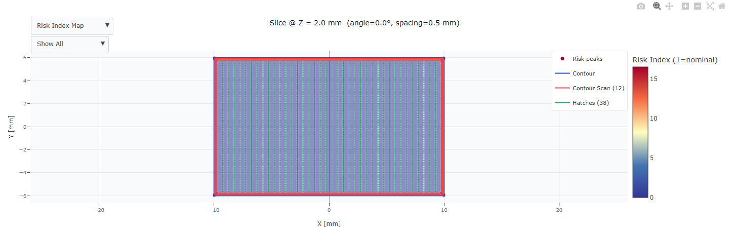
The calculation converts the spatial section into local two-dimensional coordinates. The central block section therefore appears around the local origin, approximately −10 to +10 and −6 to +6 mm. This does not move the uploaded part. Read slice position from the input and path positions in the plot's reference frame.
The upload offers STL and OBJ; the dimension display uses millimetres. The upload service checks file extension and a 50 MiB limit. A formally accepted file may still contain open surfaces, unsuitable units or no valid section. A single closed mesh with known bounds is a better starting point than an unchecked assembly.
Back to top ↑Chapter 04Setting complete inputs with their units
This Python module declares fixed input and output roles. Use the field reference to distinguish constraints from results. The flexible role assignment offered by some traditional LV equation modules does not automatically apply here. In particular, V12–V15 are outputs; a target time is addressed by changing scan speed.
The complete teaching-case input table is:
| Field | Input | Unit / selection |
|---|---|---|
| V1 · Slice Plane | 3 | Z Plane (XY cross-section) |
| V2 · Slice Position | 2 | mm |
| V3 · Hatch Angle | 0 | ° |
| V4 · Hatch Spacing | 0.5 | mm |
| V5 · Scan Speed | 1000 | mm/s |
| V6 · Hatch Laser Power | 200 | W |
| V7 · Contour Scan Speed | 800 | mm/s |
| V8 · Contour Laser Power | 150 | W |
| V9 · Layer Thickness | 40 | µm |
| V10 · Material | 1 | Inconel 718 |
| V11 · Beam Diameter | 0.08 | mm |
| V16 · Sigma Override (visual) | 0 | mm |
| V17 · Overhang Sensitivity | 0 | – |
The main unit traps
- Layer thickness V9 uses micrometres: 40 µm is 0.04 mm. Do not enter 0.04 into a field displaying µm.
- Beam diameter, hatch spacing and slice position are in mm; scan speeds are in mm/s.
- Laser powers are in W. Power and energy are not interchangeable quantities.
- Angle is a geometric input; material selection and beam diameter affect the thermal visualization assumption, not automatically the fixed contour offsets.
These process numbers are deliberately teaching parameters for investigating the software. They establish no suitable machine strategy for Inconel 718 or AlSi10Mg. Do not treat them as manufacturing approval.
Back to top ↑Chapter 05First calculation: one layer of the block
The aim is to understand geometry and assessment through an easily checked section. A block without holes or overhangs simplifies verification: section area must be 20 × 12 = 240 mm² regardless of hatch angle or speed.
- Open your own Additive chapter and upload the demonstration STL.
- Check the 20 × 12 × 4 mm bounds.
- Select the Z plane and Z = 2 mm, then enter all values from the inputs chapter.
- Confirm inputs and wait for a completed calculation without errors.
- Check V15 first, then the path plot and finally V12/V13/V14.
- Compare against the reference table only with matching geometry and parameters.
| Case | V12 segments | V13 hatch length [mm] | V14 hatch time [s] | V15 area [mm²] |
|---|---|---|---|---|
| Base | 38 | 433.2 | 0.4332 | 240 |
| Half speed | 38 | 433.2 | 0.8664 | 240 |
| Wider spacing | 19 | 216.6 | 0.2166 | 240 |
| Rotated hatching | 44 | 442.39 | 0.4424 | 240 |
Reference values were obtained on 7 September 2026 by directly executing the unchanged module source. Interpreter, dependencies and source hash are recorded in the execution report. That report does not establish the Python package versions installed on your Web server.
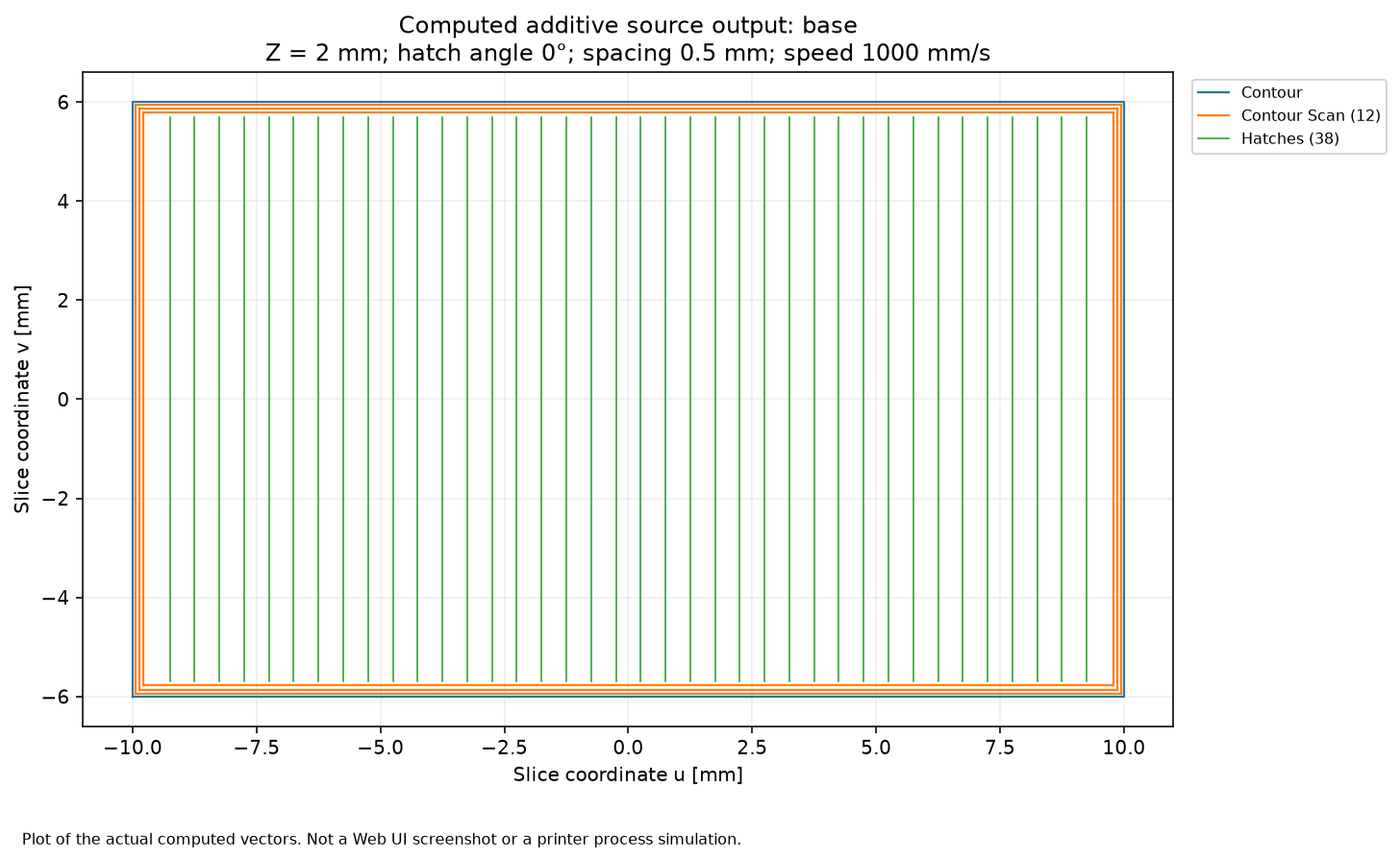
The base case produces 38 hatch segments and 433.2 mm of hatch length. At 1,000 mm/s this gives 0.4332 s. The area and this simple time check can be followed independently. Exact segment count also depends on contour offsets, boundary treatment and library version.
Chapter 06Comparing angle, spacing and speed
Return to the base input set before each change. This makes the effect of each parameter identifiable. The example includes three separate variants with unchanged mesh and slice plane.
| Variant | Change | Observation and meaning |
|---|---|---|
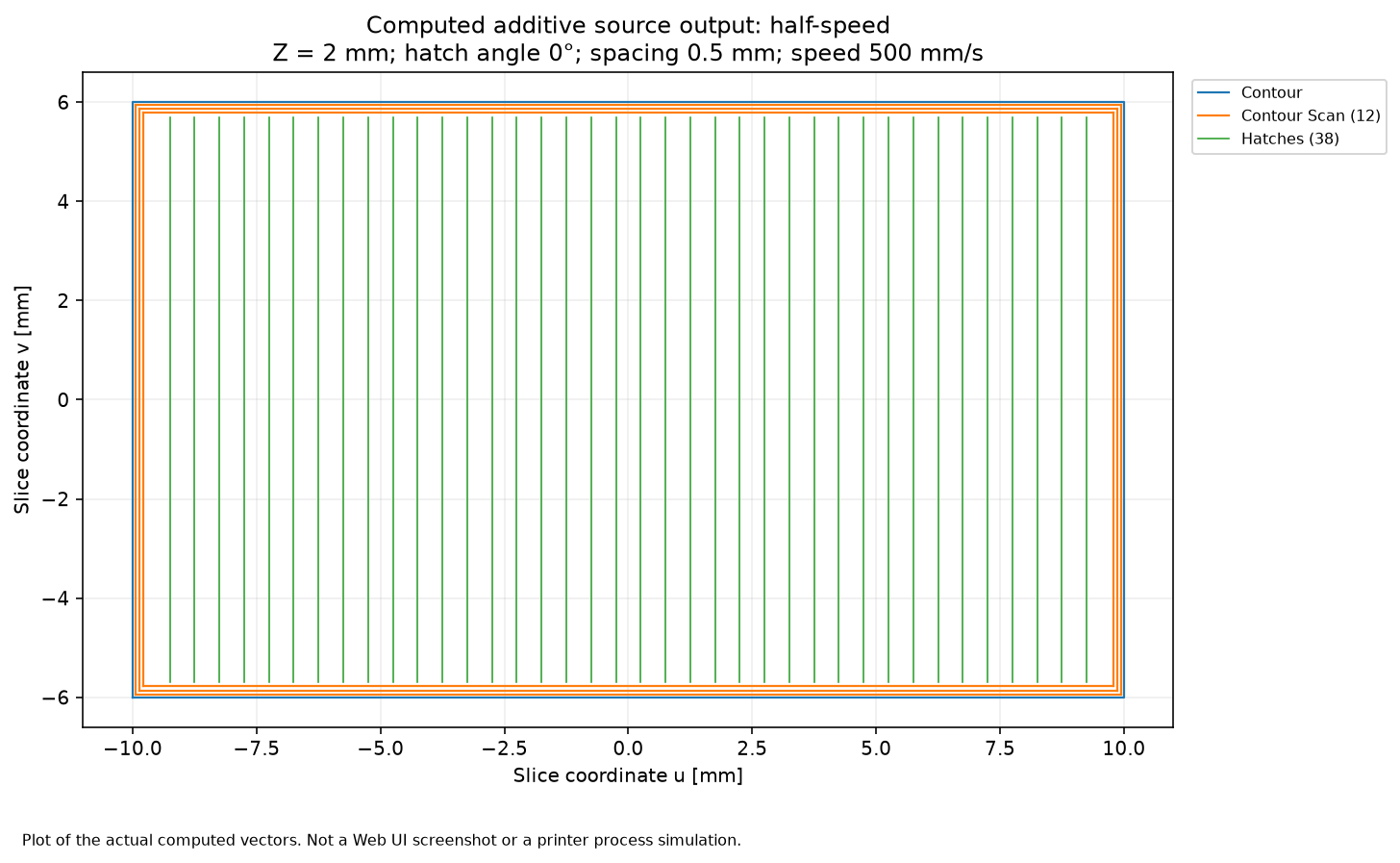
| Half speed | V5: 1,000 → 500 mm/s | Path count and length remain unchanged; reported time doubles to 0.8664 s. |
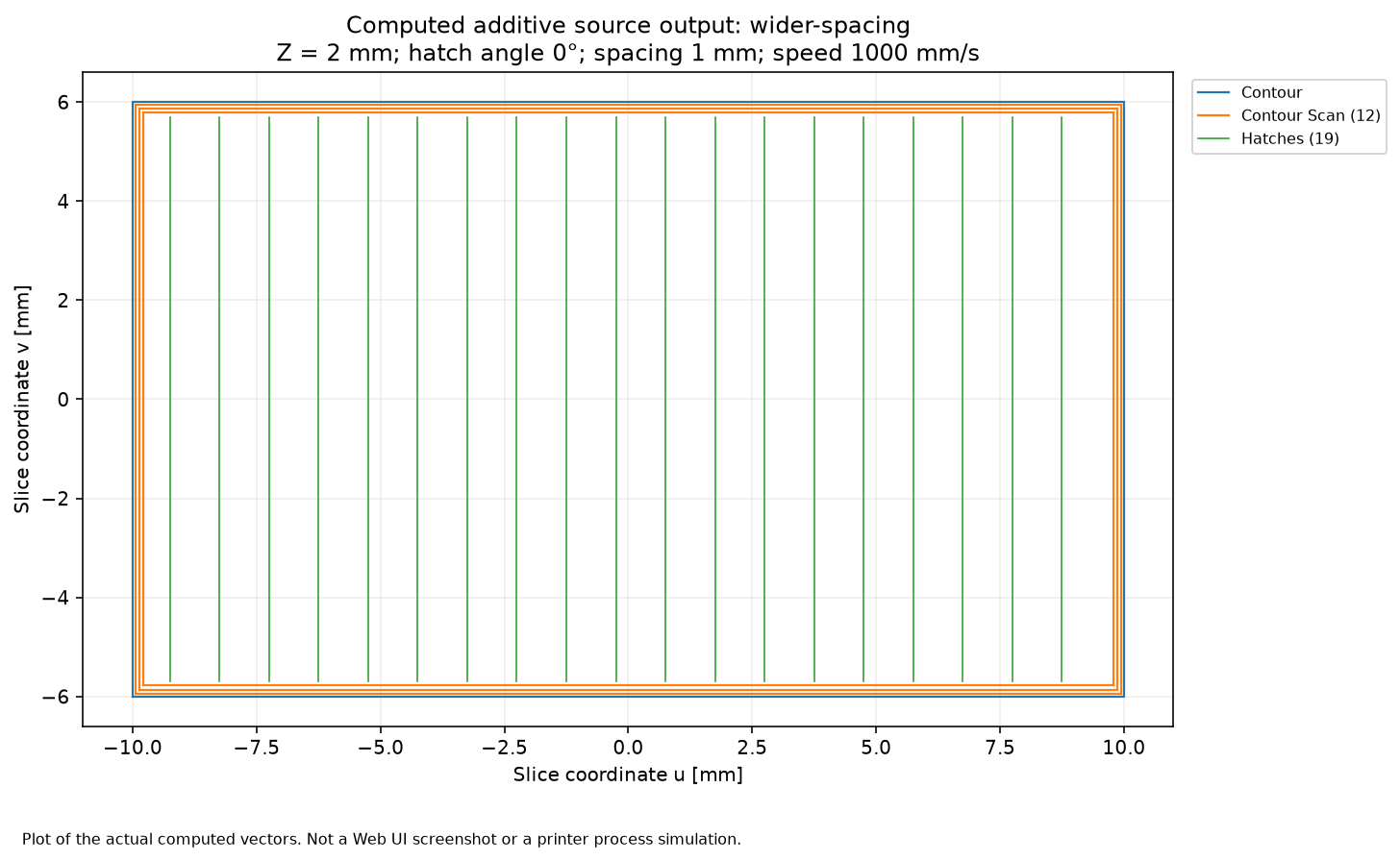
| Wider spacing | V4: 0.5 → 1 mm | 19 rather than 38 segments, 216.6 mm length; fewer paths do not establish adequate melting. |
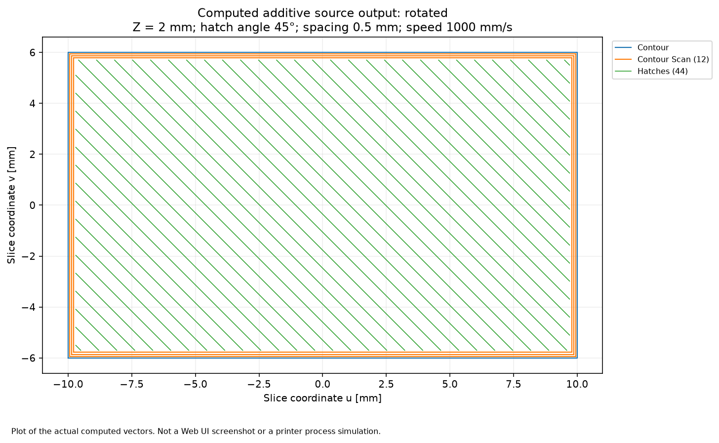
| Rotated hatching | V3: 0 → 45° | 44 segments and 442.39 mm length; area remains 240 mm². |
The angle comparison shows why “number of lines × part width” is not generally sufficient. Oblique paths encounter the boundary after different distances. Actual length is summed from the individual segments. A nominal hatch line through a part with holes may split into several separate segments.
Examine contours as well as metrics. Lower reported time is not a sufficient optimization objective if boundary coverage or process requirements are lost. Record every unchanged quantity in the variant table, including material, powers and layer thickness.
Chapter 07Investigating a target time through speed
You want to determine the hatch speed corresponding to a target reported scan time. Keep mesh, slice, angle and spacing unchanged. Hatch length L then remains constant in this calculation route, giving the algebraic relationship v = L / t.
For the base case with L = 433.2 mm and a target of 0.8664 s, v = 500 mm/s. Enter that speed in V5 and recalculate. The executed comparison confirms 0.8664 s with unchanged length. You have adjusted an input; V14 has not become a freely prescribed solver input.
- Record current path length and all geometry/hatch parameters.
- Define a positive target time for exactly the reported time component.
- Calculate v = L/t using mm and s.
- Set V5 and verify that generated path length remains unchanged.
- Assess changed power/speed ratios separately.
Chapter 08Distinguishing contours, hatches and time components
The plot contains the geometric section boundary, actual contour scan paths and hatching. These lines serve different purposes. The section boundary describes geometry. Contours are offset inward; hatching fills the remaining region. Hatch segments therefore stop short of the original rectangular boundary.
The inspected source sets two inner and one outer contour, 0.06 mm spot compensation and a 0.08 mm additional hatch offset. These are implementation parameters, not separate input fields in this module. V11 “Beam Diameter” does not change them automatically.
What V13 and V14 omit
V13 sums hatch segments only; V14 uses that length and V5. Contour scanning, jumps, acceleration, settling, recoating and other layers are not included as complete machine time. Although V7 is contour speed and affects contour-related energy visualization, it is not used to add contour time to V14.
Label this quantity “reported hatch time” in your report. Estimating machine time requires separate modelling or measurement of additional time components and the actual execution strategy.
Back to top ↑Chapter 09Interpreting the risk visualization
The coloured view is based on generated paths and their energy weighting. Hatch and contour contributions depend on quantities including P/v. The source distributes them on a grid and applies Gaussian smoothing as a simplified spatial spreading assumption. It derives an energy-density view and a dimensionless comparison index.
An index near 1 denotes the model's nominal process reference. It is neither a temperature of 1 °C nor a general verification of pore-free melting. Internal names such as temp_z likewise do not establish a physically resolved temperature calculation. Interpret the quantity through its documented calculation, not colours or variable names alone.
Material and smoothing
V10 selects between the property sets embedded in the source for Inconel 718 and AlSi10Mg. That does not fully address temperature dependence, batch variation or process approval. Conductivity, density, heat capacity, beam diameter and speed determine a characteristic smoothing width. V16 can explicitly override this width for visualization.
The teaching case verifies the four numerical path results. It does not quantitatively validate the risk index against thermal measurements or a melt-pool experiment.
Back to top ↑Chapter 10Overhangs and unavailable supplementary maps
V17 controls overhang sensitivity. When enabled, the source examines support below the current layer and uses it as an additional factor in the risk model. In the inspected implementation, investigation depth is ten times the entered layer thickness. At 40 µm this is 0.4 mm.
The teaching case deliberately sets V17 to zero, disabling that supplementary assessment and simplifying path verification. The block case therefore validates neither an overhang assessment nor a support strategy. Extending it requires suitable geometry, a defined build orientation and an independently assessable expectation.
Check path results and supplementary maps separately
Support-map and hotspot-map creation are supplementary steps whose failure does not necessarily abort the calculation. A missing map may therefore coexist with available path results. Read messages and inspect the layers actually displayed. Successful path results do not establish that every supplementary analysis was available.
If changing only V17 produces a markedly different picture, first check build axis, slice position and layer thickness. Visualization sensitivity does not replace mechanical assessment of supports or distortion.
Back to top ↑Chapter 11Using the plot, scan animation and CSV
When plot data are available, the Web interface provides an interactive visualization. Start with contours and hatching to understand the section geometry, then switch between available maps or layers. Keep view bounds and scale consistent when comparing variants.
The “Scan” button visualizes the supplied path order; “scan_path.csv” exports path information. The generated animation path places contour segments before hatch segments. This visualization differs from reported time V14 and does not establish a complete representation of machine kinematics.
Before sharing
- Does slice position match the case being discussed?
- Are contour and hatch layers visible, or has one been hidden?
- Is the active colour map clearly identified as energy density or index?
- Are sigma override and overhang sensitivity documented?
- Does the exported file correspond to the last successful calculation?
This handbook's images show the actual calculated path vectors as original plots from the documented source execution. They are not reconstructed Web masks. The local two-dimensional axes are explicitly labelled as slice coordinates.
 123
123- The selectors switch between the available visualizations.
- Boundary, contour scan and the 38 hatch segments are separate traces.
- The colour scale shows a dimensionless risk index, not temperature.
Original capture dated 7 September 2026: the unchanged application chart renderer displays actual computed data in an isolated preview. Not a complete module mask or a Web-session test. Open original
Chapter 12Saving the project and mesh together
Save the calculation under a clear name and also retain the original STL/OBJ file. The inspected upload service tracks mesh files temporarily within sessions. This does not establish that a saved project permanently embeds the geometry.
- Record module version, mesh filename, mesh hash and geometric bounds.
- Save all inputs from the field reference with their units.
- Export required path data and a plot with a readable legend.
- Reopen a project copy and inspect the upload area.
- If geometry is missing, explicitly upload the same original file again.
- Compare slice area, path count, length and time only after successful recalculation.
An old result with no mesh is insufficient for reproducibility. A same-named mesh may also contain different geometry bytes. The teaching case therefore pins its exact original with a SHA-256 hash.
The available evidence covers direct source execution and static handbook checks. A Web save/reload roundtrip has not been newly tested. The steps above describe the check for your own project state.
Back to top ↑Chapter 13Resolving common situations
Start by checking the last successful input set. Change one item at a time during diagnosis and read the message after the next calculation attempt.
No calculation without a mesh despite “Optional” in the header?
The current source requires a file. Upload your demonstration STL to the correct instance.
The slice is empty.
Compare axis and position against the bounding box. Z=5 mm is outside the block.
Area differs from the data sheet.
Check scale, axis, position, holes and mesh geometry before changing hatch parameters.
Zero degrees does not produce the expected direction.
Check the angle convention in the actual plot. The generated direction in local section coordinates is decisive.
Slice coordinates are negative.
The 2D section transformation uses a local origin. Distinguish mesh bounds from local plot coordinates.
Hatching stops short of the boundary.
Contour and hatch offsets create this clearance. It is not automatically a geometry error.
More lines but not proportionally more length?
Oblique boundaries or holes create segments of different lengths. V13 sums their actual lengths.
Changing contour speed does not affect V14.
V14 uses hatch length and V5 only. Contour time is not added.
Half speed gives double time.
That matches L/v when path length is unchanged. Also assess the changed energy input.
The risk index is being read as temperature.
The dimensionless map is a comparison model; internal temp names and colours do not establish a measured temperature.
Sigma override makes the image smoother.
You are changing a smoothing assumption. This does not establish reduced real thermal peaks.
Path values exist but a supplementary map is missing.
Read messages. Supplementary maps can fail without aborting the overall path calculation.
A reopened project has no geometry.
Check temporary upload state and reload the same original STL; retain the mesh alongside the project.
A same-named file produces different results.
Compare hashes. A filename alone does not establish identical mesh bytes.
The module reports missing dependencies.
Have the operator check the Python runtime and installed module dependencies. Changing a result target does not fix this.
An output cannot be prescribed.
The module has fixed field roles. Calculate V5 for a target time, then verify the result.
The mesh upload is rejected.
Check STL/OBJ extension, file size and readable geometry. The inspected upload limit is 50 MiB.
Values differ slightly from this handbook.
Compare source and library versions with the execution report; segment/boundary handling can depend on version.
Chapter 14Reference for all 17 fields
Identifiers come from the inspected Python module descriptor, version 1.4.0. They are not mapped from an outdated function-header comment that starts result numbering earlier; the descriptor and actual assignments V12–V15 establish the result fields.
| Identifier | Field name | Role / unit | Meaning |
|---|---|---|---|
| V1 | Slice Plane | Input · – | Select the section normal direction. 1: X Plane (YZ cross-section) · 2: Y Plane (XZ cross-section) · 3: Z Plane (XY cross-section) |
| V2 | Slice Position | Input · mm | Position inside the detected mesh bounds. |
| V3 | Hatch Angle | Input · ° | Hatch direction in the local section. |
| V4 | Hatch Spacing | Input · mm | Spacing between adjacent hatch paths; must be positive. |
| V5 | Scan Speed | Input · mm/s | Speed used for reported hatch time. |
| V6 | Hatch Laser Power | Input · W | Power weighting hatch energy input. |
| V7 | Contour Scan Speed | Input · mm/s | Contour speed for contour energy visualization. |
| V8 | Contour Laser Power | Input · W | Power weighting contour paths. |
| V9 | Layer Thickness | Input · µm | Layer thickness in µm; also used for overhang investigation depth. |
| V10 | Material | Input · – | Simplified property set embedded in the source. 1: Inconel 718 · 2: AlSi10Mg |
| V11 | Beam Diameter | Input · mm | Beam diameter for spreading assumption; does not automatically set contour offsets. |
| V12 | Number of Hatch Lines | Output · – | Number of generated hatch segments, excluding contours. |
| V13 | Total Path Length | Output · mm | Sum of hatch-segment lengths, despite the general source label. |
| V14 | Estimated Scan Time | Output · s | Hatch length / V5; not complete layer time. |
| V15 | Slice Area | Output · mm² | Net area of the current section; holes are accounted for geometrically. |
| V16 | Sigma Override (visual) | Input · mm | A positive input overrides smoothing width for visualization. |
| V17 | Overhang Sensitivity | Input · – | Zero disables the support map; larger values weight it in the model. |
Chapter 15Sources, evidence and next steps
The single configured package member is identified by its Python descriptor and its handling in the Web component. The source record contains inspected files and hashes. The execution report records four successful variants, two controlled error cases, interpreter and library versions.
Execution used the unchanged calculation source in a separate local environment. That provides more evidence than a merely described numerical example, while remaining limited to that path: no new Web upload, browser calculation, machine control, thermal validation or metallurgical process validation.
Primary references
- PySLM: Hatcher API — contour offsets, hatch spacing and angle.
- PySLM: Slicing and Hatching — the relationship between closed section boundaries, contours and hatching.
Library documentation explains its role. This example is governed by the versions recorded in the execution report and the parameters actually set. A controlled geometry with a hole or overhang is the next useful learning case before investigating a complex assembly.
Back to top ↑