Engineering task and calculation objective
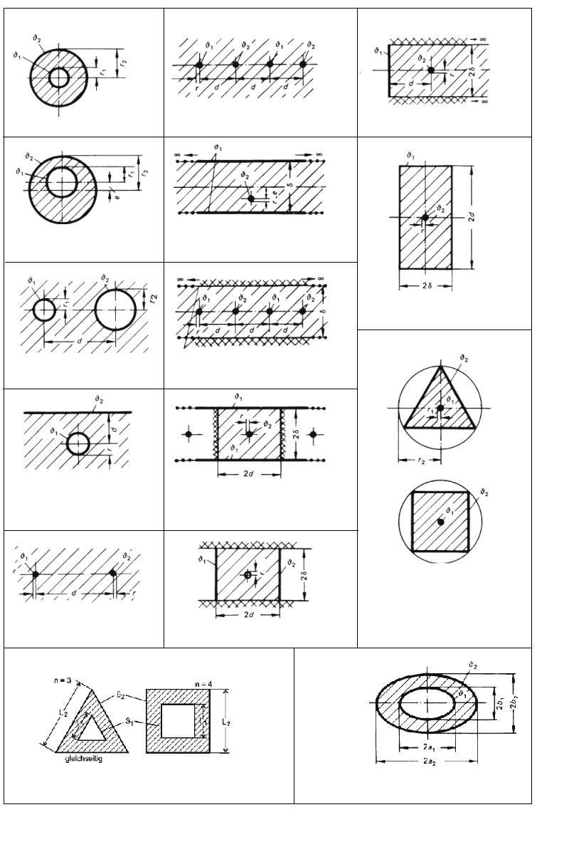
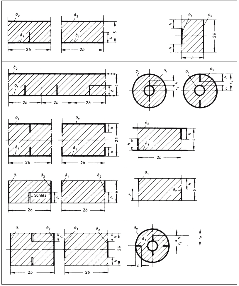
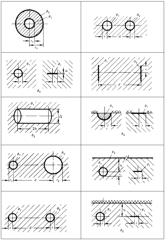
This module calculates steady-state heat conduction according to the VDI Heat Atlas (VDI-Wärmeatlas, 12th edition 2019) for the classic basic geometries: plane walls and plates, hollow cylinders (pipes), and hollow spheres – each also in multilayer form – as well as fins, rods, and wires. In addition, two-dimensional conduction problems can be handled via shape factors, for example buried pipes or bodies with oval and rectangular cross-sections.
Calculating steady-state heat conduction is one of the fundamental tasks of equipment and plant engineering: temperature profiles in vessel and furnace walls, heat flows through pipe walls and insulation layers, the effectiveness of fins on heating and cooling surfaces, or the wall temperatures of multilayer structures. From thermal conductivity, layer thickness, and area, the conduction resistance of each layer is obtained; the series connection of the resistances yields the heat flow and the intermediate temperatures.
The module follows the relations from section E1 of the VDI Heat Atlas and provides the results in a form that can be used directly in overall heat transfer and heat loss calculations (for instance with the module for the heat loss of walls and pipework).
Standard and calculation basis: VDI-Wärmeatlas, 12. Auflage 2019
Calculation workflow
- Define the geometry: First, the basic geometry is chosen: plane wall, hollow cylinder, or hollow sphere, in single or multilayer form – alternatively a fin, a rod, or a two-dimensional case with a shape factor. The geometry determines which conduction equation is applied.
- Specify dimensions and material properties: For each layer, the thickness or the inside and outside diameters and the thermal conductivity at the governing mean temperature are entered. For temperature-dependent conductivity, the value at the mean layer temperature is used, which may require a short iteration.
- Set the boundary conditions: The surface or wall temperatures on both sides, or a prescribed heat flow, serve as the thermal boundary conditions. This fully determines the steady-state conduction problem.
- Calculate the resistances and the heat flow: For each layer, the conduction resistance is formed – proportional to the thickness for the plane wall, with the logarithm of the diameter ratio for the hollow cylinder, and with the difference of the reciprocal radii for the hollow sphere. The series connection yields the total resistance and from it the heat flow.
- Evaluate the temperature profile and special cases: From the heat flow and the individual resistances, the temperatures at the layer boundaries follow. For fins and rods, the fin efficiency and the temperature profile along the fin are additionally calculated; for two-dimensional cases, the heat flow is determined via the shape factor of the arrangement.
Input quantities
| Quantity | Symbol | Unit |
|---|---|---|
| Area | A | m² |
| Wall temperature 1 | ϑ0 | °C |
| Wall temperature 2 | ϑn | °C |
| Number of layers | n | – |
| Layer 1 | s1 λ1 | m |
| Layer 2 | s2 λ2 | m |
| Layer 3 | s3 λ3 | m |
| Layer 4 | s4 λ4 | m |
| Layer 1 | r1 λ1 | W/(m·K) |
| Layer 2 | r2 λ2 | W/(m·K) |
| Layer 3 | r3 λ3 | W/(m·K) |
| Layer 4 | s4 λ4 | W/(m·K) |
| Layer 1 | ϑ1 | °C |
| Layer 2 | ϑ2 | °C |
| Layer 3 | ϑ3 | °C |
| Layer 4 | ϑ4 | °C |
| X-coordinate | x | m |
| Beginning of layer All coordinates refer to x = 0 | xk | m |
| Thermal conductivity | λk | W/(m·K) |
| Temperature at beginning | ϑk | °C |
| Length | l | m |
| Inside | r0 | m |
| Layer 1 | r1 λ1 | m |
| Layer 2 | r2 λ2 | m |
Calculated results
| Quantity | Symbol | Unit |
|---|---|---|
| Heat flux per length unit | Q/l = Ql | W/m |
| Thermal conductivity | λ | W/(m·K) |
| Shape factor | Sl | - |
| Temperature | ϑ2 | °C |
| Temperature | ϑ1 | °C |
| Calculation according to VDI Heat Atlas table number | Tafel | - |
| Configuration number | Anordnung | - |
| b1 | b | m |
| Delta | δ | m |
| a1 | a c | m |
| c | a c | m |
| n | n | - |
| h | h | m |
| e | e | m |
| d | d | m |
| b2 | b1 b2 | m |
| a2 | a1 a2 | m |
| Shape factor | Sr | - |
| r | r | m |
| r1 | r1 r2 | m |
| r2 | r1 r2 | m |
| Circular disk / sphere | Kreisscheibe | - |
| _Bemerkung | _Bemerkung | - |
| _Bemerkung | _Bemerkung | - |
Calculation options
Circular disk / sphere
Circular disk · Sphere
Worked example
A pipe is insulated with a 50 mm thick mineral wool shell. The insulation starts at the pipe outside diameter of 88.9 mm; its surface temperatures are 150 °C on the inside and 40 °C on the outside. The thermal conductivity of the mineral wool at the mean temperature is 0.05 W/(m·K). Find the heat flow per unit length through the insulation layer.
Given values
| Inside diameter of the insulation layer d1 | 88.9 mm |
| Outside diameter of the insulation layer d2 | 188.9 mm |
| Inner surface temperature ϑ1 | 150 °C |
| Outer surface temperature ϑ2 | 40 °C |
| Thermal conductivity λ | 0.05 W/(m·K) |
Solution
Formula for the hollow cylinder
For steady-state heat conduction through a cylindrical layer, the heat flow per unit length is:
ql = 2 · π · λ · (ϑ1 − ϑ2) / ln(d2/d1)
Insert the diameter ratio
ln(d2/d1) = ln(188.9 / 88.9) = ln(2.125) = 0.7537
Calculate the heat flow
ql = 2 · π · 0.05 W/(m·K) · (150 − 40) K / 0.7537
ql = 34.56 / 0.7537 W/m ≈ 45.9 W/m
About 46 W per meter of pipe thus flow through the insulation layer. The temperature profile within the layer is logarithmic over the radius.
Result
| Heat flow per unit length q_l | ≈ 45.9 W/m |
All values are illustrative. The applicable standard and project-specific boundary conditions remain authoritative.
Frequently asked questions
When may I calculate steady-state, and when do I need a transient analysis?
Steady-state calculation requires that the boundary conditions do not change with time, or only slowly compared with the thermal time constant of the component. This is satisfied for continuous operating states of furnaces, pipework, and vessels. Start-up and shutdown, batch processes, or upset scenarios, on the other hand, require a transient analysis, because there the heat storage in the wall dominates the behavior.
Why is the logarithm of the diameter ratio used for a pipe?
In a hollow cylinder, the area available for heat flow grows with the radius, so the heat flux decreases toward the outside. Integrating the Fourier equation over the radius therefore yields the resistance R = ln(d_a/d_i)/(2·π·λ·L) per pipe length. The approximation using a mean area is permissible only for thin-walled pipes; for thick-walled layers such as insulation it leads to significant errors.
How do I deal with contact resistances between the layers?
The ideal series connection assumes full-area contact between the layers. Real interfaces – for instance between a pipe and a slipped-on insulation shell, or between a wall and its cladding – have air gaps that act as an additional resistance. In insulation calculations, this usually acts favorably (more resistance), but in cooling tasks it is dangerous, because the heat removal is overestimated. When in doubt, contact resistances should be applied conservatively.
What does the fin efficiency express?
The fin efficiency is the ratio of the heat flow actually dissipated through the fin to the heat flow the fin would dissipate if it were entirely at the base temperature. It decreases with increasing fin height, increasing heat transfer coefficient, and decreasing thermal conductivity of the fin material. Long, thin fins made of poorly conducting material therefore add hardly any extra duty – fin design is always an optimum between area and efficiency.