Fluid Properties – Thermophysical property calculations
Define fluids and states unambiguously, operate H2O and GLYC, and transfer consistent property sets.
No chapter found. Try another search term.
Chapter 01Which properties does your calculation need?
A heat exchanger calculation can converge neatly with an incorrect viscosity and still represent the wrong operating point. A seemingly small mistake in composition or pressure reference affects density, heat transfer and pressure loss. This handbook explains how to define a fluid state unambiguously, select the appropriate module and transfer a consistent set of properties.
The learning path starts with water in H2O and a glycol mixture in GLYC. It then considers gases, humid air, solutions and user tables. The module map covers all 25 configured package members. Detailed field-level instructions cover H2O and GLYC; the other modules receive engineering selection guidance, but not yet a complete individual manual.
You need the identity of the fluid, its state and the intended use of the data. “Water at 80 °C” is not a complete specification for a dependable property set: pressure, phase and any saturation assumption must agree. “Glycol, 35%” leaves even the product and concentration basis unresolved.
Read the preparation and both examples first. Then use the field reference and troubleshooting as a reference path. Example numbers are explicitly identified historical regression expectations from May 2026. Images are approved WTS demonstration captures from September 2026 illustrating the transition to the consuming calculation; they are not new H2O or GLYC mask captures.
Back to top ↑Chapter 02From process conditions to a reviewed property set
- Define the task: Do you need a heat balance, pipe-flow calculation, boiling point or phase equilibrium? Record which property is required in which equation.
- Identify the fluid: Pure substance, specified commercial product or mixture? Preserve its composition and data source.
- Define the state: Temperature, absolute pressure, phase and any composition or humidity. Distinguish inlet, outlet and property evaluation temperature.
- Select the module and calculate: Enter the physical driving data. Allow dependent properties to be calculated.
- Review the results: Compare units, magnitude, state and relationships between the resulting quantities.
- Transfer and recheck: Transfer or connect the complete relevant property set; then make a controlled change to a driving input.
This sequence is a working procedure. It does not mean every property must always remain an output. A suitable inverse calculation may, for example, determine concentration from freeze protection. The number of independent specifications must still match the task, and the module must support the requested direction.
An automatic child chapter and a separately created property chapter are different routes. In the former, the parent module manages transfers. In the latter, you establish provenance, units and update behaviour yourself. State explicitly in the project description which route you use.
Conceptual workflow diagram. Automatic, variable-linked and manual transfers are established separately in each chapter.
Back to top ↑Chapter 03Module map: all 25 package members
This table preserves the exact identifiers in package configuration. Some routes supply properties directly; others determine composition, a dew point or retrieve data from an external source. Shared package membership does not make these tasks interchangeable. Listed ranges come from the inspected module descriptions; they do not constitute new validation of the underlying correlations.
| Module and task | Required data | Results / use | Limit and learning path |
|---|---|---|---|
| Bier Wort and beer | Temperature and composition appropriate to the product. | Properties for thermal calculations. | Catalogue range 0–75 °C; do not extend it to arbitrary food products. |
| CO2 Carbon dioxide | Temperature, absolute pressure and single-phase or boiling state. | State-dependent properties. | Distinguish liquid, vapour and critical region; read the domain for the selected route. |
| EGAS Natural gas | Gas composition; use L/H presets only when appropriate to the analysis. | Gas properties for flow and heat transfer. | A preset is not a measurement of the delivered gas quality. |
| FRIG Refrigerants | Exact fluid/mixture designation and thermodynamic state. | Refrigerant properties for the selected route. | The list is limited; do not equate similar trade names or new mixtures. |
| GLYC Antifrogen L, N, KF, SOL | Product route, temperature and an appropriate composition or freeze-protection specification. | Density, heat capacity, viscosities, conductivity and further product quantities. | Detailed instructions and historical composition comparison in this handbook. Worked case |
| H2N2 Fixed hydrogen-nitrogen mixture | Temperature and pressure for the catalogue composition of 98 volume% H2 / 2 volume% N2. | Properties of that gas mixture. | Do not confuse it with N2H2; the reversed identifier denotes a different module route. |
| H2O Water and steam | State pair, absolute pressures, saturation selection and quality x where required. | Thermodynamic and transport properties, with separate saturation phases. | Detailed instructions and historical pressure comparison; not a universal property module for all aqueous solutions. Worked case |
| H2SO Sulphuric acid-water | Pressure, temperature, composition and phase being examined. | Phase equilibrium and available properties. | Read concentration basis and phase values together; pure-water properties do not replace solution data. |
| HCL Hydrochloric acid-water | Pressure, temperature and composition. | Properties of the HCl-H2O system. | Do not transfer results to another acid merely because concentration is similar. |
| HE Helium gas | Temperature and absolute pressure. | Properties in the gas range described by the catalogue. | Catalogue: 20–1500 °C and 1–100 bar; no liquid-helium cryogenic route is established here. |
| HNO3 Nitric acid-water | Pressure, temperature, composition and phase task. | Phase equilibrium and properties. | Use consistent state data for both phases; this is not independent approval across every concentration range. |
| HX Humid gases and mixing | Temperature, pressure and a clearly defined humidity basis; both streams for mixing. | State quantities and mixing of two humid gas streams. | Distinguish relative humidity and water loading; do not mix dry and humid mass bases. |
| N2H2 Multicomponent gas mixture | Fractions of available N2, O2, H2, CO, CO2, H2O, SO2 and SO3 components. | Properties assuming all components are gaseous. | Partial condensation is not included according to the catalogue. |
| NaOH Sodium hydroxide solution | Temperature and NaOH mass concentration. | Properties of the aqueous solution. | Catalogue range 20–100 °C and 0–50 mass%; entering a number does not extend applicability. |
| OEL Machine oils | Appropriate viscosity grade and temperature; identify the actual product. | Viscosities, density, conductivity, heat capacity and Prandtl number. | A viscosity grade does not fully characterize every oil product. |
| PROP Interface to PROPER | Available external data source and its required fluid/state definition. | Properties obtained through the supported interface route. | Installation and availability were not tested live here; no REFPROP connection is claimed. |
| RGAS Flue gas from fuel data | Lower heating value and measured CO2 content; select fuel type. | Statistically calculated flue-gas composition and associated property route. | Do not equate this with a full measured gas analysis or VGAS inputs. |
| SAC Sucrose-water | Temperature and concentration on the module basis. | Properties of a sucrose-water solution. | Catalogue source: sugar atlas; not evidence for arbitrary sugar or food mixtures. |
| SaWa Seawater | Temperature and salinity in the specified unit. | Salinity-dependent properties. | Catalogue: 0–180 °C, 0–150 g/kg; do not reuse a percentage value unchanged. |
| SCUT Multicomponent distillation | Component system, separation task and specifications required by the actual module. | A distillation route assigned to the package. | The reviewed source identifies only the task; detailed operation and current Web access require separate verification. |
| SDAT Free property input | Complete data set with state, units, source and applicability. | Manually specified values for further calculations. | Entry alone does not establish physical validity or temperature dependence. |
| SODM Sodium | Fluid state and module-specific temperature/pressure conditions. | Properties for the sodium route. | Sodium is not sodium hydroxide solution; do not substitute NaOH or water data. |
| STAB User property tables | Reviewed table with temperature/pressure axes and units. | Read or interpolated properties for receiving modules. | Check table boundaries and interpolation behaviour; do not assume extrapolation. |
| TSO3 Acid dew point | SO3 and H2O fractions on the required gas basis. | Acid dew point for the described flue-gas route. | Acid dew point and water dew point are different quantities. |
| VGAS Combustion calculation for gases | Fuel-gas composition and supported combustion conditions. | Stoichiometric air/flue-gas quantities and combustion relationships. | Catalogue: up to ten components; incomplete combustion at air ratio below 1 is not included. |
The configuration also includes historical or specifically integrated routes. Check actual availability in your module selector. Detailed H2O/GLYC instruction does not replace the outstanding individual manuals for the other identifiers.
Back to top ↑Chapter 04Prepare the fluid, state, basis and provenance
Create a small data specification for each stream: unique name, composition, concentration basis, inlet and outlet conditions, pressure reference, expected phase, property model and source. This prevents a colleague from interpreting the same number differently when checking the calculation.
For mixtures, distinguish mass fraction, mole fraction and volume fraction. Write, for example, “GLYC, 1,2-propylene glycol/Antifrogen L model, mass fraction 0.35” rather than “glycol 35”. Commercial products contain additives; identifying the main constituent does not establish equivalence with every available formulation.
Also check the selected module's applicable range. An input mask may display a numerical range while an individual property correlation has a narrower domain. An accepted input establishes neither that the fluid remains liquid nor that all reported properties are supported equally well throughout that range.
Create a separate example project. Give chapters descriptive names such as “Water – pressure comparison at 80 °C” and “GLYC L – composition comparison at 20 °C”. The two state columns initially represent two evaluation points. Your specification makes them inlet/outlet or before/after. Two different concentrations must not inadvertently become the supposedly unchanged fluid at opposite ends of a closed circuit.
Back to top ↑Chapter 05Pressure and units: the most common mix-ups
Use absolute pressure to determine a thermodynamic state. If a gauge measures pressure relative to the surroundings, pabs = pgauge + pambient. Ambient pressure is a separate boundary condition. Merely changing the display from Pa to bar does not add atmospheric pressure.
1 bar = 100,000 Pa and 1 MPa = 10 bar. The water example therefore uses 100,000 Pa to mean 1 bar absolute. The second column's 2 bar corresponds to 200,000 Pa. Typing “1” into a field still labelled Pa specifies a completely different state. Confirm an input with its unit or select the display unit first, then read the value back.
The reviewed H2O and GLYC module definitions use mPa·s for dynamic viscosity and m²/s for kinematic viscosity. In SI calculations, 1 mPa·s = 0.001 Pa·s and 1 mm²/s = 10−6 m²/s. Changing units and converting dynamic viscosity into kinematic viscosity are different operations; the latter requires density.
Temperature differences have the same numerical value in K and °C. An absolute temperature in a gas equation requires kelvin. Enthalpy and heat capacity may be displayed in J or kJ; document this factor as carefully as the pressure reference.
Back to top ↑Chapter 06Understand what the properties do
Density ρ relates mass and volume flow. Heat capacity cp describes the temperature dependence of specific enthalpy at constant pressure. Thermal conductivity λ describes heat conduction through the fluid. Dynamic viscosity η relates shear stress to velocity gradient; kinematic viscosity ν relates it to density.
Three relationships help review the results: ν = η/ρ, a = λ/(ρ cp) and Pr = η cp/λ = ν/a. Use η in Pa·s and cp in J/(kg·K). Apply a tolerance appropriate to the rounded source values; a discrepancy in the last displayed digit does not establish a calculation defect.
Enthalpy h and entropy s use a model reference state. In an energy balance, take consistent differences from the same data basis. Equal temperatures at different pressures do not necessarily imply identical enthalpies. A negative enthalpy alone is insufficient evidence of an error because reference states differ.
Surface tension and heat of evaporation describe an interface and a phase transition, respectively. Do not blindly treat these as single-phase liquid properties. Speed of sound is not the operating fluid velocity in your equipment. A field's name and physical meaning matter more than a familiar symbol.
Back to top ↑Chapter 07Liquid, vapour or saturated: establish the state first
For a single-phase pure fluid in an appropriate domain, two independent state variables, such as temperature and pressure, determine the state. At liquid-vapour saturation, temperature and pressure are linked: specifying saturation pressure makes saturation temperature a result. Quality x is an additional specification for the mixture of saturated phases.
Each H2O column has a “Calculation for saturation?” setting (V21/V22). On the saturation route, leave either temperature or pressure free. Do not prescribe an arbitrary pressure and an independent temperature as simultaneous fixed saturation data. Liquid and vapour results appear in separate groups; they are not interchangeable approximations for the same fluid.
For wet steam, x is the vaporized mass fraction, not volume fraction. Between the saturation limits, specific enthalpy obeys h = h′ + x(h″ − h′). This does not justify arbitrary averaging of viscosity or heat-transfer coefficients. At x = 0 the state is saturated liquid; at x = 1 it is saturated vapour. Superheated vapour is not simply represented by x greater than 1.
In the historical water example, 80 °C at either 1 or 2 bar absolute is in the liquid region. The stored result gives a boiling temperature of approximately 99.606 °C at 1 bar. This specific comparison is more useful than the inaccurate rule that water always boils at 100 °C.
Back to top ↑Chapter 08Open modules, read the columns and set driving inputs
Open the Fluid Properties package through module selection and search for H2O or GLYC. Whether a module opens in your installation depends on licensing, installed version and registration. The package map documents configured membership; it is not evidence of entitlement.
H2O shows two state columns with temperature, pressure and saturation selection, followed by result groups. GLYC also has two columns and a shared fluid selection V87. The reviewed selection is 1 = 1,2-propylene glycol/Antifrogen L, 2 = ethylene glycol/Antifrogen N, 3 = Antifrogen KF and 4 = Antifrogen SOL. Use the readable names in everyday work; the numbers here establish precise source identity.
Initially work from top to bottom. Confirm each value and inspect its returned unit. Distinguish a value just entered, a persistent lock and a field supplied by a connection. Colour helps orientation but does not replace field information about provenance and role.
Do not also lock calculated outputs merely to “secure” them. That creates additional constraints and makes later temperature or composition changes harder. Before an inverse calculation, release exactly the specification that should become the unknown; after a fluid selection change, reconsider inherited concentrations and product-specific limits.
Back to top ↑Chapter 09First worked case: water at 80 °C and two pressures
Purpose and evidence
Compare two liquid states at the same temperature. This reveals changes caused by pressure and explains why “water properties at 80 °C” does not fully replace pressure. Numbers come from the stored H2O regression reference of 15 May 2026. They were not recalculated in a running application for this handbook. The exact plugin version used then is not documented.
Enter the data
- Open H2O in a separate demonstration project and name the chapter appropriately.
- Set “Calculation for saturation?” to No in both columns (V21/V22 = 0).
- Set both temperatures T1 and T2 to 80 °C (V1/V2).
- Enter p1 = 1 bar absolute and p2 = 2 bar absolute (V3/V4; internally 100,000 and 200,000 Pa).
- Run the calculation. Leave density, heat capacity, conductivity, viscosities and enthalpy free as outputs. Check the resulting liquid state; do not manually copy internal region identifiers or fluid constants.
Historical comparison values
| Property | State 1 | State 2 | Unit |
|---|---|---|---|
| Density | 971.8023 | 971.847 | kg/m³ |
| Heat capacity | 4195.5186 | 4195.2993 | J/(kg·K) |
| Thermal conductivity | 0.66698855 | 0.66704184 | W/(m·K) |
| Dynamic viscosity | 0.3540578 | 0.35408458 | mPa·s |
| Kinematic viscosity | 3.643311e-7 | 3.6434193e-7 | m²/s |
| Prandtl number | 2.227109 | 2.2269828 | − |
| Enthalpy | 334990.53 | 335070.12 | J/kg |
Density rises only from about 971.802 to 971.847 kg/m³ here. Enthalpy also changes despite the unchanged temperature. This observation belongs to this particular liquid state; it is not general permission to ignore pressure in gases, near saturation or around the critical region.
About 0.1% is sufficient as a reading comparison for the principal tabulated properties. This is an editorial plausibility threshold, not model uncertainty. For a larger difference, first check units, saturation selection, state and program version. The original fixture tolerance is recorded separately in the example evidence. A historical target alone does not demonstrate a successful current calculation.
Back to top ↑Chapter 10Change H2O: temperature, saturation and inverse calculation
Save the pressure comparison first. For a temperature comparison, retain both pressures at 2 bar absolute and change only T2. Then review density, viscosity, heat capacity and phase in the second column. The first column is the reference. This handbook contains no newly observed target numbers for that modified configuration.
A particularly clear change of direction is saturation calculation: in a copy, select saturation for state 1, prescribe pressure and leave T1 free. The historical pressure reference records 99.605934 °C as boiling temperature at 1 bar. The operating sequence with the saturation setting changed was not freshly executed here; after changing it, inspect both saturation phases and the expected temperature.
For the reverse direction, prescribe the saturation temperature just obtained and release pressure. With both values locked, you are checking a specified point rather than finding a pressure. An old manual connection can supply a hidden constraint just as a field lock can.
H2O source contains relationships involving different state quantities and region-dependent evaluation. This does not promise that any arbitrary combination of h, s, ρ, p and T can be inverted from every starting state. Begin a more demanding inverse calculation from a known state, change one target in small steps and inspect the phase region. If the solution moves to another region or remains unknown, return to the saved forward case and investigate the constraints first.
Back to top ↑Chapter 11Second worked case: composition at the same temperature
Purpose and inputs
Assess a cooling circuit at 20 °C. First compare two mixture concentrations to understand their effects. This is a comparison of alternatives, not a claim that concentration changes that way between the inlet and outlet of an unchanged circuit. The basis is a stored GLYC reference from 6 May 2026.
- Open GLYC and select 1,2-propylene glycol/Antifrogen L (V87 = 1; reference design type 1).
- Set T1 = T2 = 20 °C (V1/V2).
- Enter mass fraction g1 = 0.50 in column 1 and g2 = 0.35 in column 2 (V5/V6). If the display uses percent, these correspond to 50% and 35%.
- Leave volume fraction and freeze protection free. They are alternative descriptions of composition and must not also be independently locked.
- Calculate, read the concentration basis back and compare results.
| Property | State 1 | State 2 | Unit |
|---|---|---|---|
| Volume fraction | 0.48682928 | 0.3381086 | − |
| Freeze protection | -31.539272 | -16.47305 | °C |
| Density | 1044.4897 | 1033.8394 | kg/m³ |
| Heat capacity | 3563.6057 | 3827.139 | J/(kg·K) |
| Thermal conductivity | 0.38589144 | 0.4440917 | W/(m·K) |
| Dynamic viscosity | 6.8712697 | 3.9968235 | mPa·s |
| Kinematic viscosity | 0.00000657859 | 0.0000038660005 | m²/s |
| Prandtl number | 63.454365 | 34.444233 | − |
Here, 50 mass% corresponds to approximately 48.683 volume%, while 35 mass% corresponds to approximately 33.811 volume%. Treating the two percentage bases as identical would be an input error. In the stored example, the lower mass fraction yields lower viscosity and higher heat capacity, but also a less negative freeze-protection temperature. None of those quantities alone determines the appropriate mixture.
The reference values are historical expectations; neither a new run nor an independent current manufacturer comparison was performed here. Use them as a traceable training comparison. Obtain application conditions, mixing-water quality and minimum concentration for the actual purchased product from its accompanying manufacturer documentation.
Back to top ↑Chapter 12Specify freeze protection and release concentration
The practical question is often: which concentration gives an agreed freeze-protection temperature? GLYC explicitly contains relationships between mass fraction and freeze protection for L and N. The source accounts for releasing a previously derived concentration when freeze protection becomes a new specification.
- Copy the saved GLYC L forward case. Retain the fluid and T1 = 20 °C.
- Release mass fraction g1. Do not additionally lock volume fraction.
- Initially use the unrounded freeze-protection value V27 from your own forward calculation as the inverse target. The historical reference value is −31.539272 °C.
- Recalculate and check whether g1 returns to approximately 0.50. Then inspect V27, g1, v1 and the remaining properties together.
- Only after this direction check, investigate a modified freeze-protection specification within the product range.
This is a reproducible test procedure derived from source; this edition does not include a freshly observed GLYC inverse run. When you perform it, record actual values, units, locks, messages and program version. Returning to the expected mass fraction checks the direction within the selected model, not complete product approval.
Distinguish freeze protection from the lowest operating condition of the entire installation. Cold-start viscosity can constrain a pump or flow more severely than the fluid's temperature limit. Therefore repeat property evaluation at the actual lowest operating temperature. The two numbers in the 20 °C comparison do not replace that cold-start case.
Back to top ↑Chapter 13Distinguish L, N, KF and SOL correctly
GLYC is not a single universal glycol equation. Selection switches between product routes with their own composition and temperature conditions. L uses the propylene glycol route, N the ethylene glycol route. KF denotes an aqueous formate solution and is not another name for L. SOL has a separate product route in the inspected source; its concentration is not intended to vary freely like an L/N mixture.
The reviewed GLYC-1 mask contains conditional groups for all four selections. The separate GLYC-2, GLYC-3 and GLYC-4 mask files are empty. Those file names therefore do not establish four independently verified user interfaces. The operating explanation follows the visible fluid selector and the fields actually displayed after selection.
Source limits for mass fraction extend to 0.6126 for L and 0.6432 for N; volume fractions have different limits. The KF route uses a lower volume-fraction limit of 0.314. These are limits of the inspected calculation route, not a recommendation for mixing fluid for an installation. Product requirements may be narrower.
Product names also evolve. The current manufacturer's range lists SOL HT, for example. Do not equate a current commercial name with the historical SOL model route without checking. The manufacturer's overview helps identify products; it does not establish that the module implements the latest formulation or data edition.
Back to top ↑Chapter 14Check the numbers: units, dimensionless groups and duty
The stored values allow consistency checks independent of the operating interface. For the first GLYC state, use η = 6.8712697 mPa·s = 0.0068712697 Pa·s and ρ = 1044.4897 kg/m³. This gives ν ≈ 6.57859·10−6 m²/s, consistent with stored V15.
For H2O, η = 0.3540578 mPa·s and ρ = 971.8023 kg/m³ give a kinematic viscosity of approximately 3.64331·10−7 m²/s. The factor of 1000 between mPa·s and Pa·s is crucial. This handbook automatically checks these algebraic relationships; no plugin is executed by those checks.
An additional teaching calculation illustrates heat capacity. Hypothetically prescribe 2 kg/s mass flow and a 10 K temperature rise for both GLYC alternatives. If cp is simplified by holding it at its 20 °C value, Q̇ = ṁ cp ΔT gives approximately 71.272 kW at g = 0.50 and 76.543 kW at g = 0.35. These numbers are newly derived hand calculations using historical properties, not a WTS design.
For a real calculation, use the appropriate enthalpy difference or a justified mean heat capacity over the actual temperature interval. Lower viscosity alone does not guarantee a particular pressure loss: geometry, flow regime and volume flow also matter. Do not directly compare water at 80 °C with GLYC at 20 °C as though only the fluid had changed.
Back to top ↑Chapter 15Supply properties to WTS and follow changes
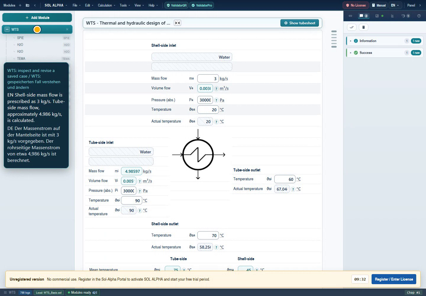
WTS needs tube-side and shell-side fluid properties. The visible H2O child chapters in the historical water/water example show a real relationship in a saved project. Their chapter numbers depend on the project. The second H2O is not automatically “state 2” of the first; it is a separate module call.
 123
123Unmodified frame from the approved WTS demo video of 6 September 2026. This is the WTS parent mask, not a newly captured H2O/GLYC mask. Historical numbers are not a recommended operating point.
- Two H2O child chapters are visible in the WTS project tree. Associate each with the correct stream.
- The parent mask explicitly labels pressure as absolute. Units and pressure reference must agree.
- Mass flow and volume flow are different quantities. A property change can alter their relationship.
For an ordinary WTS fluid route, select the fluid in WTS and then inspect the corresponding child chapter. Read the transferred temperatures, pressure and any concentration. Establish which values originate in the parent before manually replacing a connected value. An overwritten child field may be supplied again on the next parent calculation.
For deliberately prescribed properties, prepare a transfer list containing ρ, cp, λ and η or ν, their associated states and units. One new density combined with old viscosities does not constitute a consistent fluid change. Select the intended data route in the receiving module; this handbook does not claim automatic linkage of arbitrary independently created H2O/GLYC chapters.
Then change just one driving quantity, such as temperature. Trace the change from the WTS input through the correct property child to heat transfer, duty and pressure loss. Leave a managed child value unchanged when it demonstrably belongs to a different evaluation location. The WTS worked case describes complete heat-exchanger operation.
Back to top ↑Chapter 16Which temperature belongs to which property?
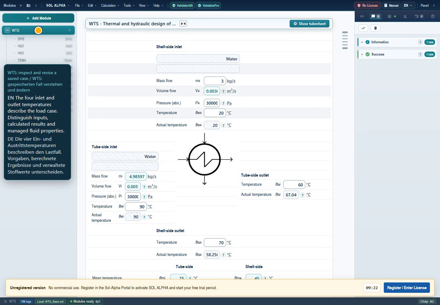
A heat exchanger has inlet and outlet temperatures for both streams. Subcalculations may additionally require properties at mean fluid temperature or wall temperature. These evaluation locations have different engineering meanings. The WTS mask distinguishes specifications, actual temperatures and further evaluation values.
 123
123Unmodified frame from the approved WTS demo video of 6 September 2026. This is the WTS parent mask, not a newly captured H2O/GLYC mask. Historical numbers are not a recommended operating point.
- Inlet and outlet conditions belong to different process locations.
- Specified and recalculated temperatures are displayed separately in this historical WTS mask.
- Property evaluation temperatures are below the main visible area. Do not substitute arbitrary inlet values for them.
Before each transfer, ask whether this value serves an energy balance, local heat transfer or a hydraulic state. A balance needs consistent inlet and outlet enthalpies. A heat-transfer method may require separate viscosities at fluid and wall temperature. Density used to convert an actual volume flow belongs to the conditions at that flow measurement.
Image captions and licence notices form part of the historical capture and remain visible. In particular, do not adopt the displayed pressures as recommended boundary conditions: the figure teaches field provenance and state assignment, not an approved real operating point. Your own calculation requires actual absolute pressures and phase checks.
When comparing fluids, initially hold temperature, pressure and comparison basis constant. Deliberately choose whether mass flow or volume flow remains unchanged. They are equivalent at equal density but usually not during a fluid change. Record the selected basis with the variant result, so that an apparent improvement is not simply caused by altered boundary conditions.
Back to top ↑Chapter 17Gases, flue gas and humidity: choose the correct basis
For gases, pressure directly affects density. Along with temperature and absolute pressure, record whether a quantity denotes mass, amount of substance, operating volume or standard volume. Standard volume flow requires defined standard conditions. Changing a displayed m³/h quantity into kg/h is not merely a scaling operation without fluid state and data basis.
For EGAS, choose an appropriate composition. Available L/H variants are characteristic starting points. When using an actual analysis, included components and concentration basis must match the input. Check the total and document whether unknown residual components were excluded, added or deliberately grouped. This handbook does not claim universal automatic handling of residual components.
According to the reviewed description, N2H2 treats every component as gaseous. Water or acid condensation is therefore outside that premise. HX treats humid-gas states and mixtures; distinguish relative humidity from water loading and quantities per kg dry gas from those per kg humid gas. The same numerical value can imply a different balance on another basis.
VGAS starts from fuel-gas composition to determine combustion relationships. RGAS instead uses a statistical route involving heating value and a CO2 measurement. TSO3 answers the specific acid-dew-point question. A workflow diagram may connect these modules conceptually without claiming an automatically configured data channel.
Back to top ↑Chapter 18User properties, tables and external sources
SDAT is the route for deliberately prescribed properties. STAB reads values from user-defined tables. PROP is described in the catalogue as an interface to PROPER. These are different tasks: individual free input, a temperature/pressure-based table and an external data route. Neither the local PROP installation nor a complete Web roundtrip was verified for this edition.
Check a table first at an existing data point and then between points. Record axes, units and number format. Test boundary behaviour before calculating outside the table. A table reader cannot correct missing phase boundaries or wrong fluid names by producing a numerically smooth curve.
For imported data, include the fluid, composition, model, edition and reference state in the report. In particular, do not combine absolute enthalpies from two different data sources without review. For η and ν, verify the unit and corresponding density. Columns of numbers without state and units are not a complete property set.
NIST REFPROP is an example of an independent thermophysical reference database with fluid/mixture selection and state conditions. Mentioning it does not claim an existing SOL ALPHA integration. An independent comparison is meaningful only when fluid, composition, phase and units actually agree.
Back to top ↑Chapter 19Study alternatives without mixing comparison conditions
State a question before creating a parameter series: how does GLYC viscosity change with temperature at unchanged composition? Or how do heat capacity and freeze protection change at unchanged temperature? Both questions are useful, but require different quantities to remain fixed.
Start with a few individually reviewed points. Save fluid, composition basis, pressure and locks. Change only the intended variable in each comparison. In a temperature series, composition and product route remain unchanged; in a composition series, temperature and other state assumptions remain unchanged. Changing fluids requires its own comparison and newly checked domains.
Inspect every point for warnings and phase changes. A continuous line between valid endpoints does not prove that the intervening path is single-phase or valid everywhere. For large temperature intervals, explicitly include evaluation points near operating limits, such as cold start and maximum fluid temperature.
For a later program-driven study, use the study function available in your installation and read its actual generated points back. This handbook provides no unverified universal entry syntax or claim of an already executed H2O/GLYC series. In the report, distinguish measured data, model values and simplified teaching calculations, and identify the quantities deliberately held constant.
Back to top ↑Chapter 20Save, reopen and verify the data route
Save forward cases as separate project states before performing inverse calculations. Record fluid, conditions and comparison purpose in the description. A meaningful name such as “GLYC L 20 °C – 50/35 mass% – historical comparison” is more useful for later review than an unlabelled result list.
Reopen the saved example in a separate session. First inspect the visible values without changes: are product selection, units, locks, both state columns and connections retained? Recalculate only afterwards. This distinguishes the saved state from newly produced results.
For a WTS connection, inspect chapter structure and the origin of transferred properties. Make a small driving change and follow whether the expected child chapter and its consumers update. An unchanged display immediately after opening does not alone establish a working connection.
This handbook edition does not document a freshly executed H2O/GLYC save/reopen check. The historical number reference and WTS context images serve different evidential purposes. Your own reopening test should record program version, file, steps, numbers and messages; the checklists make that test reproducible without declaring it passed in advance.
Back to top ↑Chapter 21Review results and hand them to other calculations
Review the property set in three steps before transfer. First: is the fluid unambiguous and is the model appropriate? Second: do state, phase, units and concentration basis agree? Third: are results and dependencies consistent with expectations? Only then is a result list meaningfully usable.
Compare ρν with η after unit conversion. Check cp, λ and Pr for magnitude and mutual consistency. For an energy balance, verify the enthalpy reference; for gas flows, distinguish standard and operating volume; for solutions, verify the composition basis; for humid gas, distinguish dry and humid mass bases.
Record actual data provenance in each receiving chapter: automatic child module, explicit variable connection, manual transfer, user table or external source. Describe a change check so a later user knows which consumers require review when conditions change.
A useful handover identifies both data and limits: “H2O, liquid, 80 °C, 1 bar absolute, η in mPa·s; historical reference from May 2026, current replay still pending” is transparent. For real project approval, replace the pending replay with your documented execution and include the receiving module's engineering requirements. A general successful-calculation status does not replace this provenance check.
Back to top ↑Chapter 22Look up H2O and GLYC fields
This selection covers 67 concrete identifiers in related pairs. “V1 / 2” means V1 for state 1 and V2 for state 2. Units are the reviewed module units; the interface may use different display units. Roles depend on the situation and are not a universal input/output list. Internal helper fields are not presented as user entries that must be filled in.
H2O
| Fields | Quantity | Source unit | Meaning and role |
|---|---|---|---|
| H2O: V1 / 2 | Temperature | °C | Driving input in the ordinary p/T case; may be a saturation result. |
| H2O: V3 / 4 | Absolute pressure | Pa | Pressure associated with temperature; explicitly convert bar displays. |
| H2O: V21 / 22 | Saturation selection | − | Links pressure and temperature at saturation. |
| H2O: V5 / 12 | Density | kg/m³ | Upper result block; observe the displayed phase. |
| H2O: V6 / 13 | Isobaric heat capacity | J/(kg·K) | For Prandtl number and justified sensible-heat balances. |
| H2O: V7 / 14 | Thermal conductivity | W/(m·K) | Fluid property; not a heat-transfer coefficient. |
| H2O: V10 / 17 | Dynamic viscosity | mPa·s | Multiply by 0.001 before using SI check equations. |
| H2O: V9 / 16 | Kinematic viscosity | m²/s | ν = η/ρ using properties at the same state. |
| H2O: V11 / 18 | Prandtl number | − | Transport ratio; not direct verification of heat transfer. |
| H2O: V19 / 20 | Enthalpy | J/kg | Use consistent differences for energy balances. |
| H2O: V41 / 42 | Entropy | J/(kg·K) | Retain the reference state and phase. |
| H2O: V23 / 29 | Vapour density | kg/m³ | Separate vapour block at saturation. |
| H2O: V35 / 36 | Vapour enthalpy | J/kg | Distinguish it from the liquid value. |
| H2O: V37 / 38 | Heat of evaporation | J/kg | Difference between saturation enthalpies. |
| H2O: V54 / 55 | Vaporized mass fraction | − | Only within the corresponding two-phase model. |
| H2O: V56 / 57 | Wet-steam enthalpy | J/kg | Mixture value using quality x. |
| H2O: V60 / 61 | Thermal expansion coefficient | 1/K | Not universally restricted to positive values. |
| H2O: V78 / 79 | Speed of sound | m/s | Not the equipment flow velocity. |
| H2O: V96 / 97 | Specific volume | m³/kg | Reciprocal of density at the corresponding state. |
| H2O: V108 / 109 | Thermal diffusivity | m²/s | a = λ/(ρ cₚ) as a consistency check. |
GLYC
| Fields | Quantity | Source unit | Meaning and role |
|---|---|---|---|
| GLYC: V87 | Fluid | − | Shared L/N/KF/SOL selection for both columns. |
| GLYC: V1 / 2 | Temperature | °C | Evaluation temperature of the respective composition. |
| GLYC: V5 / 6 | Mass fraction | − | 0.35 means 35 mass%; alternative specification to volume fraction. |
| GLYC: V7 / 8 | Volume fraction | − | Do not equate it numerically with mass fraction. |
| GLYC: V27 / 28 | Freeze protection | °C | Possible inverse target for supported products. |
| GLYC: V9 / 10 | Density | kg/m³ | Combine with viscosity at the same state. |
| GLYC: V11 / 12 | Heat capacity | J/(kg·K) | Depends on temperature and composition. |
| GLYC: V17 / 18 | Thermal conductivity | W/(m·K) | Transfer together with the remaining properties. |
| GLYC: V13 / 14 | Dynamic viscosity | mPa·s | Observe the factor of 1000 relative to Pa·s. |
| GLYC: V15 / 16 | Kinematic viscosity | m²/s | Do not read as mm²/s without conversion. |
| GLYC: V19 / 20 | Prandtl number | − | Model ratio; rounded individual values yield an approximation. |
| GLYC: V23 / 24 | Boiling temperature | °C | Interpret only for the selected product route. |
| GLYC: V25 / 26 | Vapour pressure | Pa | Not an independent operating-pressure specification. |
| GLYC: V85 / 86 | Thermal diffusivity | m²/s | Check against λ, ρ and cₚ at the same state. |
Chapter 2320 practical troubleshooting questions
Start from the observed situation. Change one possible cause at a time and preserve a saved working starting case.
The module does not calculate although temperature and pressure are visible.
Check that values are actually known and confirmed, which units apply and whether saturation is selected. An unknown result placeholder differs from a dependable specification; field information establishes its role.
Why does density change for the same water?
Density belongs to a state. Compare temperature, absolute pressure, phase and evaluation location. Equating different states is not a statement of constant fluid properties.
I have 1 bar gauge pressure. What belongs in H2O?
Add actual ambient pressure and enter the result as absolute pressure. Changing units from bar to Pa does not change the pressure reference.
50% glycol does not give 0.50 in the other concentration field.
Mass and volume fractions differ. In the historical L example, mass fraction 0.50 gives volume fraction approximately 0.486829. Also check whether the display shows fraction or percent.
Why is dynamic viscosity different by a factor of 1000?
The reviewed H2O and GLYC definitions use mPa·s. Divide by 1000 for calculations in Pa·s. The numerical value alone is insufficient for comparison.
Can I copy ν directly into the η field?
No. Use η = ρν with consistent SI units at the same evaluation location. The units have different dimensions.
Prandtl number does not match every digit of my hand calculation.
Use unrounded data and correct units. Individual properties may come from separate correlation routes. Distinguish a small difference from a unit error; document substantial discrepancies.
Why does H2O show two result groups?
At saturation, liquid and vapour properties can appear separately. Columns represent states; vertical groups represent phases. Select the value appropriate to the receiving calculation.
May vapour quality exceed 1?
In the described wet-steam model, x is a mass fraction between 0 and 1. Superheated vapour requires a single-phase state route and is not represented by x greater than 1.
Inverse concentration calculation remains blocked.
Release mass fraction and alternative composition specifications while freeze protection is prescribed. Check the fluid and its range. Start with your own forward value.
GLYC KF displays different fields from L.
Product selection changes the model route. KF is a formate solution; L is the propylene glycol route. Do not reuse an L concentration as a KF input without checking.
Can I dilute SOL arbitrarily with water?
The inspected SOL route does not treat freely variable concentration like L/N. Establish the actual product and manufacturer instructions; a different SOL commercial product is not automatically the same model.
WTS overwrites a property in a child chapter.
Check the field source. In a managed child route, the parent may transfer values again. Change the driving specification at its intended location.
After changing fluids, a result remains suspiciously similar.
Check that all relevant properties updated and no old manual locks remain. Updated density combined with old viscosities can create a mixed data set.
Why should I not use the gas-mixture route below the dew point?
The reviewed N2H2 description assumes all components are gaseous and excludes partial condensation. Below the relevant dew point that premise no longer holds; select a suitable phase route.
Is H2N2 the same as N2H2?
No. H2N2 denotes a fixed 98/2 volume mixture of hydrogen and nitrogen in the catalogue. N2H2 is a different multicomponent gas route. Read the task description rather than reinterpreting the letters.
Can I multiply standard volume flow by operating density?
Only after converting to the same reference conditions. Standard and operating volume flows belong to different temperatures and pressures. Explicitly record the standard conditions.
Why does my table differ from a built-in module?
Compare fluid definition, reference state, units, interpolation and applicability. A similar fluid name does not establish identical data. Save the table and version reference with the project.
Can I adopt historical targets as current results?
The tables document an earlier reference. Recalculate the case in your installation, record differences and review the basis. Copying a target value does not test a solver.
What should be saved with the project?
Fluid, composition and basis, states, source and model version, units, roles/locks, connections, result comparison and outstanding checks. For tables or external data, include their exact edition.
Chapter 24Terms for a dependable property comparison
| Term | Meaning |
|---|---|
| State | Consistent thermodynamic conditions of an unambiguously defined substance. |
| Evaluation location | Physical or representative location whose temperature and pressure belong to a property value. |
| Mass fraction | Mass of a component divided by total mass. |
| Volume fraction | Volume-based composition with defined reference conditions; not generally identical to mass fraction. |
| Absolute pressure | Pressure referenced to vacuum. |
| Saturation | Consistent liquid-vapour equilibrium state with linked pressure and temperature. |
| Quality | Vaporized mass fraction in the described two-phase model. |
| Dynamic viscosity | Property η, also often called μ; the source modules use mPa·s. |
| Kinematic viscosity | ν = η/ρ; the source modules use m²/s. |
| Transport property | Property such as viscosity or conductivity describing momentum or heat transport. |
| Reference state | Specified reference basis, for example for enthalpy and entropy. |
| Model domain | Conditions for which a model or correlation is intended. |
| Historical evidence | Stored earlier state; no claim of a current recalculation. |
| Managed child chapter | Calculation route called and supplied with data by a parent module. |
Chapter 25Sources, image provenance and reviewed scope
Which version forms the basis?
Web: main13.0 / 1cd12e8b173ba72aa5c95c98a14772b7ee537997. All-Dev: fix-iteration/v10 / 40606b705b2df95e550ffef5e98ab733ccc66229. The source inventory and file hashes document package configuration, module descriptions, H2O/GLYC masks and selected module definitions and calculation routes. Working-tree state was recorded at collection; hashes identify the actual inspected files.
H2O example values come from a repository regression reference dated 15 May 2026; GLYC L comes from a reference dated 6 May 2026. The example data and provenance include original path, SHA-256, inputs, selected expectations and units. This JSON is readable evidence, not a directly loadable SOL project. The original plugin builds are not documented; no current live run, complete Desktop/Web parity or coverage of every product variant is claimed.
Primary engineering references
- IAPWS R7-97(2012), industrial formulation IAPWS-IF97: context for the water/steam model and its separate state regions. Full IAPWS domains are not presented without verification as identical functionality in every H2O release.
- NIST REFPROP: independent reference database for pure fluids and mixtures. No built-in REFPROP interface is claimed.
- Clariant Antifrogen L and Antifrogen KF: product identity cross-check. Current product information does not replace identification of the data edition implemented in the module.
Genuine images and explicit limits
The two images are unmodified frames from the already approved WTS video of 6 September 2026. Image provenance records timestamps and SHA-256 hashes. Added numbering is separate HTML over the originals. Both images show the WTS property context, not standalone H2O/GLYC acceptance. New module captures and fresh inverse/reopening evidence remain outstanding.
The package map is complete for all 25 configured members. H2O and GLYC are the detailed teaching routes; other individual manuals, all special cases and every manufacturer product are not thereby complete. Bundled text, tables and images work offline; optional primary-source links require Internet. The manifest describes the published scope.
Back to top ↑