Pressure loss – Flow and pipe network calculations
Understand pipe losses, use RDV and NPSH with clear references, and review coupled pipe networks.
No chapter found. Try another search term.
Chapter 01From process case to hydraulic decision
This handbook moves from an individual flow path to the pump and a branched network. It helps prepare pressure-loss calculations, assign inputs correctly and assess results technically. A “pressure loss” value becomes usable only after the fluid, flow rate, temperature, geometry and balance boundary are defined. The same pipe can fulfil very different duties during a cold start, warm continuous operation and low tank level.
Where should you start?
For a heat exchanger, start with the RDV section and its transition from WTS. For a liquid pump, first read pressure references and then the NPSH workflow. A branched network also requires the topology review in the RNET chapter. The package map lists all 24 modules and separates pipe flow, control, metering, separation and supporting thermal tasks.
The examples have different evidence levels. A simple pipe example is a fully specified analytical teaching calculation. The NPSH case comes from a historical regression dataset and includes explicitly examined invalid power data. Workflows for changes, connections and reopening were prepared from sources; no new live run of these three modules was performed for this edition. Each example states this distinction.
The work product
The result should be a reviewable case description: operating point, included resistances, pressure definition, boundary conditions, acceptance limits and unresolved uncertainty. Increasing pump head may enable more flow while reducing suction margin. A thermally improved heat exchanger may perform less favourably hydraulically. Both effects belong in the decision.
Back to top ↑Chapter 02Prepare a complete calculation case
Sketch the fluid path before entering module values. Mark free surfaces, pressure connections, pump, heat exchanger, valves, branches and elevations. Give each section an unambiguous identifier. This reveals which losses RDV supplies, which piping another module covers and which boundary condition the network calculation prescribes.
- Select the operating case: Normal duty, maximum flow, cold start or minimum suction level. Flow and temperatures must be values that can occur together.
- Define the fluid: Record its name, composition, phase, density, dynamic viscosity and, where relevant, vapour pressure at the appropriate state.
- Establish geometry: Source the inside diameters, lengths, roughness, parallel paths, fittings and elevation datum.
- Separate knowns and unknowns: Decide whether flow, pressure difference or geometry is sought. A released target must not simultaneously remain prescribed by a connection.
- Calculate and review: Check units and status first, velocity and Reynolds number next, then component losses, total loss and system effect.
- Save traceably: Keep the case name, input status, sources, result and open issues together. Give each changed case its own identity.
A blank result is not a small number. An existing value can belong to a previous state. Observe the actual calculation status after every change and whether a field is prescribed, calculated or linked. Colour alone is insufficient as a permanent record of input status.
For project review, maintain a short section register: identifier, from/to, fluid state, flow, loss source and included components. This prevents double counting and makes it easier to divide a network into calculable tasks later.
Conceptual workflow diagram; actual data connections are checked for each module.
Back to top ↑Chapter 03Place all 24 modules in context
The following map matches the configured package membership. It includes pipe flow, machinery, metering, separation and supporting thermal tasks. A shared package name does not imply identical methods or code coverage. Availability depends on the actual installed modules and licence.
| Module | Task | When to use it and what to check |
|---|---|---|
| A2 | Safety-valve flow area | Establish upset flow, fluid and allowable back pressure; valve sizing is a separate protective-function calculation. Identify the code edition and certified discharge data. |
| CAV | Control valve and throttling | For liquids and gases including critical and subcritical flow. Establish valve characteristics, approach flow and reducers; a pipe loss coefficient does not replace valve sizing. |
| DKEG | Stodola steam-cone law | For the relationship between steam flow and pressure states in the appropriate machine model. Do not infer a complete turbine characteristic or general network solution. |
| DROS | Differential-pressure flow measurement | Select orifice plates, nozzles and Venturi forms by their actual construction. Distinguish metering differential pressure, permanent loss and the applicable standard limits. |
| DRRB | Crossflow finned-tube bundle | For pressure loss across a finned-tube bundle. Pitch, fins and minimum free area define the reference flow; plain-pipe friction values cannot simply be reused. |
| FDP | Adiabatic pipe flow | Compressible and incompressible flow including fittings. Track pressure level and state changes for gases; one constant liquid-style density may be insufficient. |
| FLD | Wire-mesh and fibre separator | Assess the separation duty and droplet or particle distribution together with hydraulics. A low pressure loss alone does not establish adequate separation. |
| HSA | Horizontal gravity separator | For separation with vessel geometry, liquid level and internals. Gas loading, liquid inventory and droplet entrainment jointly constrain the design. |
| HYBA | Tube-reboiler hydraulics | Hydraulic balance of a vertical tube-side reboiler. Driving head, heating, evaporation and circulation must be consistent; single-phase pipe losses alone are insufficient. |
| LOGI | Perforated plates and grids | For internals with a defined free area. Record open-area ratio, geometry and reference area before comparing loss coefficients with other components. |
| NKRE | Centrifugal-pump specific speed | To classify a pump from speed, flow and head. Observe the unit convention, number of stages and reference flow; this does not yield a complete NPSH curve. |
| NPSH | Pump system and suction margin | Detailed route: suction/discharge piping, system head, power and available NPSH. Establish the manufacturer curve and required margin separately; critically review historical invalid values. |
| RDV | Heat-exchanger tube-side loss | Detailed route: nozzles, entries/exits, turns and tube friction with property and fouling effects. Associate geometry with the correct thermal operating case. |
| RO | Orifice calculation | A separately registered orifice module. Check its actual mask and model scope before selection; the detailed DROS configuration list is not automatically attributed to RO. |
| STAK | Chimney draft and flow losses | Density differences provide natural draft while friction and internals consume it. Flue-gas and ambient temperatures therefore belong to the same operating case. |
| STOS | Liquid-pipeline surge | For surges and valve closure using the Joukowsky relationship. Check wave travel time, closure history and minimum pressures; steady losses do not verify transients. |
| TKL | Tank level and volume | For horizontal/vertical cylindrical vessels and associated heads. Supplies geometry for level scenarios; the hydraulic elevation datum still needs to be defined. |
| TSIP | Kettle-reboiler hydraulics | Hydraulic assessment of a kettle reboiler with thermal state and liquid inventory. Do not generally equate it with a vertical thermosiphon. |
| VSA | Vertical gravity separator | Assess gas/liquid loading and internals together. Construction and residence-time assumptions are decisive, not just an allowable pressure loss. |
| ZDP | Gas-liquid two-phase flow | Pipe loss for appropriate horizontal, upward or downward paths. Check phase fraction, slip, gravity and model range; average density alone does not describe these effects. |
| ZELL | Thermal distribution by cell method | Corrected mean temperature difference and temperature distribution provide thermal context. It belongs to the configured package but is not a general pipe-loss solver. |
| QKUK | Reciprocating-compressor coupling work | For specific coupling work with standard volume flow, stages and suction/recooling conditions. Distinguish standard and actual flow; a liquid-pump equation does not describe gas compression. |
| VSP | Leakage through a narrow annular gap | For narrow cylindrical annuli from geometry, properties and pressure difference. Establish gap width and surface condition carefully; small dimensional changes can have large effects. |
| RNET | Branched and meshed pipe networks | Detailed route: nodes, branches, boundary conditions and pressure profile in the graphical network plan. The conventional chapter mask does not replace this editor; host support is required. |
RDV, NPSH and RNET receive detailed treatment here. For other modules, the map supports selection and identifies the main interfaces. It does not replace their future complete individual handbooks.
Back to top ↑Chapter 04Distinguish absolute pressure, gauge pressure and loss
The most consequential pressure errors occur before calculation. Absolute pressure is referenced to vacuum; gauge pressure is referenced to a specified ambient pressure. A pressure difference initially means the difference between two pressures on the same reference. Irreversible flow loss represents loss of mechanical energy; measured static pressure differences may also contain elevation and velocity terms depending on the measurement locations.
pabs = pg + patm · hL = ΔpL / (ρg)
In the reviewed NPSH module, V4 and V14 are the suction- and discharge-vessel gauge pressures. V11 is barometric pressure. The source equations add V11 to the vessel gauge pressures and include elevation and losses to calculate absolute pump-nozzle pressures V19 and V20. Vapour pressure V2 is absolute. Entering an already absolute vessel pressure in V4 counts atmospheric pressure twice.
The NPSH source offers a relationship between atmospheric pressure and site altitude V8. This is a model; it does not replace a project requirement for minimum local atmospheric pressure. Also establish whether suction elevation is positive when the liquid surface is above the pump datum. Positive flooded-suction elevation increases available suction head in the documented NPSH route.
Practical cross-check
Mark every pressure source as “absolute”, “gauge” or “differential”. Convert bar and kPa into Pa before an independent check: 1 bar = 100,000 Pa and 1 kPa = 1,000 Pa. The WTS operating mask explicitly marks pressures as absolute; account for this when transferring data to NPSH. A shared unit of Pa does not prove a shared pressure reference.
Back to top ↑Chapter 05Keep flow and properties consistent
Mass flow is conserved in steady piping without additions or withdrawals. Volume flow also depends on density. During heating, cooling or appreciable gas expansion, the same volume flow must therefore not be used everywhere without a state reference. Determine the free flow area from inside diameter; nominal size and outside diameter are not equivalent.
V̇ = ṁ / ρ · v = V̇ / A · Re = ρvD / μ = vD / ν
Dynamic viscosity μ or η and kinematic viscosity ν are different quantities. The reviewed RDV and NPSH modules use dynamic viscosity in mPa·s. For the SI equation above, multiply that numerical value by 0.001 to obtain Pa·s. Kinematic viscosity is expressed in m²/s; 1 mm²/s equals 10−6 m²/s. A mistake can shift Reynolds number by several orders of magnitude.
RDV distinguishes mean fluid properties from properties at the wall state because viscosity and convection effects correct friction. This does not mean that the whole fluid is at wall temperature. In NPSH, vapour pressure, density and viscosity must belong to the pumped fluid at the considered state. The historical NPSH test in this handbook is a synthetic numerical case; it is not used to reconstruct a particular real fluid.
Obtain properties from an appropriate module described in the fluid-properties handbook or from documented project data. Mixtures also require composition and its basis. A cold glycol case can be hydraulically much more demanding than warm water at the same volume flow. One density value cannot capture that difference.
Back to top ↑Chapter 06Read Darcy, Fanning and component losses correctly
For single-phase incompressible flow in a straight circular pipe, the Darcy-Weisbach form provides a useful check equation. Fittings may be included through loss coefficients ζ, provided every coefficient uses the same explicitly defined reference velocity. This is particularly important at changes in cross-section.
ΔpL = (λD L/D + Σζ) ρv²/2 · λD = 4 fF
The two common friction definitions differ by a factor of four. In the NPSH source route, the laminar relationship 64/Re yields the Darcy factor and pressure loss contains λL/D. RDV instead calculates the isothermal coefficient using 16/Re in the laminar range and tube-friction loss using 2fρv²NPassL/D. This is a Fanning convention, with additional module-specific corrections. The letter f alone does not identify the convention.
Comparing displayed coefficients without their equations is therefore uninformative. First compare the resulting losses for identical geometry and properties. If coefficients differ by about four, check definitions before assuming a calculation defect. The NASA primary reference explicitly defines both conventions.
What should be added?
Successive irreversible losses can be combined within the same energy balance. Static-pressure recovery through an expansion and elevation pressure terms are different contributions. Parallel paths divide the flow; their losses are not added as if they were two pipes in series. Also distinguish a complete component loss from subresults already included in it.
Back to top ↑Chapter 07Assess flow regime and model limits
Reynolds number is a modelling indicator, not a universal acceptance criterion. Pipe shape, entrance conditions, disturbances and wall conditions influence transition. The reviewed NPSH implementation switches to its turbulent-friction route above Re = 2320. RDV uses its own ranges for the isothermal coefficient and further transitions for corrections. These implementation boundaries are not sharp physical boundaries for every installation.
If a result is close to a regime transition, examine at least one slightly lower and one slightly higher flow. Observe both friction factor and actual loss. A discontinuity may arise from a correlation change; conversely, a smooth curve does not prove adequate model accuracy. Record the range and chosen method in the report.
When the simple pipe equation is insufficient
For compressible gases, appreciable pressure reduction changes density and therefore velocity. Gas-liquid mixtures additionally involve slip, flow pattern and potentially hydrostatic and acceleration terms. Choose an appropriate FDP or ZDP route and review the actual module limits. Liquid-loss equations using an arbitrary average density do not generally represent these tasks.
Very narrow gaps, non-Newtonian fluids, pulsating flow, cavitation and rapid valve closure are also separate modelling decisions. VSP or STOS may suit particular tasks; module registration does not establish suitability for every special case. Clarify an uncertain physical state before selecting the calculation.
A temperature change may alter viscosity, vapour pressure and density simultaneously. Reduced pipe friction therefore does not automatically improve the NPSH case: increased vapour pressure may reduce suction margin by more.
Back to top ↑Chapter 08RDV: calculate the heat-exchanger tube side
RDV considers the tube-side flow path of a shell-and-tube heat exchanger. Its evaluation separates nozzle losses, entry/exit and turning losses, and tube friction. A fouling multiplier acts on the tube-friction contribution in the reviewed total. This helps determine whether changing the nozzle, tube area or flow arrangement is likely to be effective.
- Select the correct construction V36: straight tubes, U-tubes or bends. Associate phase V43 with the actual fluid state.
- Specify passes V13 and tubes carrying parallel flow V14 consistently. For multiple passes, do not automatically use the total tube count as the parallel count.
- Enter tube length, inside diameter, outside diameter, wall thickness and both nozzles. Do not overconstrain a geometric relationship with conflicting additional inputs.
- Associate mass flow V19 and fluid/wall properties with the same WTS operating case. Record their origin and connections.
- Calculate velocity V21, Reynolds V22 and the loss groups. Then review total V34 and its use in the overall hydraulic budget.
Δptotal = Δpnozzles + Δpentry/exit + Ft Δptube friction
In the reviewed source route this means V34 = V30 + V31 + V33·V32. V51 and V52 are separately reported nozzle subresults; do not blindly add them again to the already complete total. For a different module version, review the total actually used.
This workflow is prepared from mask and source without a new RDV live demonstration. A complete numerical first run and all construction variants remain separate execution evidence to obtain. The following simple pipe calculation provides independent orientation and is not a numerical substitute for RDV corrections.
Back to top ↑Chapter 09NPSH: work through a pump system systematically
NPSH describes the pump suction side, whereas head and power address the complete pumping duty. The module combines these quantities in one system description. Begin on the suction side because adequate discharge pressure does not remedy an inadequate pump-inlet condition.
- Name the pump and fluid in V12/V13. Define the operating point with volume flow V24.
- Specify vapour pressure V2, density V3 and pipe-calculation viscosity V25 with a defensible state description.
- Enter suction-vessel gauge pressure V4, atmospheric reference V8/V11, flooded-suction elevation V6 and any approach velocity V5 at the defined reference point.
- Describe suction piping V26–28 and its fittings V38. Calculate velocity, Reynolds number, friction factor and loss V7 where these suit the chosen calculation direction.
- Enter the discharge vessel or receiver V14/V15 and discharge piping V32–34/V39. Check head V22 against the documented elevation and pressure terms.
- Enter a justified positive pump efficiency V40. Compare available NPSH V10 with manufacturer requirement V9 and the project-specific margin.
The reviewed source route can initialize missing fitting coefficients to zero. Physically, this means no additional local losses are included there. It also initializes efficiency to zero if unknown; that state does not produce a finite usable power in the power equation. Deliberately enter the required values.
V5 and V29 are not identical merely because both use m/s. V5 belongs to the approach-flow energy reference, whereas V29 is suction-pipe velocity. For a large suction vessel, free-surface velocity may be approximately zero while pipe velocity is appreciable. State the chosen reference explicitly.
Back to top ↑Chapter 10First example: independently check a pipe
Analytical teaching calculation, not a SOL live result. Consider a horizontal circular pipe carrying steady single-phase incompressible liquid. Darcy friction factor is deliberately fixed for this exercise; it is not derived from material roughness. The calculation demonstrates scales and units, not suitability of a particular real pipe.
| Specified quantity | Value | Role |
|---|---|---|
| Actual volume flow | 0.010 m³/s = 36 m³/h | Fixed |
| Pipe inside diameter | 0.100 m | Fixed |
| Pipe length | 20.0 m | Fixed |
| Density | 1,000 kg/m³ | Fixed |
| Dynamic viscosity | 0.001 Pa·s = 1 mPa·s | Fixed |
| Darcy friction factor | 0.020 | Fixed for this teaching calculation |
| Sum of ζ | 3.0 | Reference velocity in the 0.100-m pipe |
| Pressure loss | Sought | Free |
A = πD²/4 gives A = 0.007854 m² and v = 1.27324 m/s. Reynolds number is approximately 127,324. Dynamic pressure ρv²/2 is 810.57 Pa. Pipe friction λL/D = 4 and fitting coefficient 3 combine to give a factor of 7. Thus Δp = 5,673.99 Pa = 5.674 kPa and hL = 0.57839 m at g = 9.81 m/s².
The sequence also provides a useful troubleshooting method: if velocity is wrong, check volume flow and inside area first. If Reynolds number is wrong, check viscosity conversion. If only loss is wrong, check friction convention, L/D and the ζ reference. A plausible final number can conceal two compensating unit errors, which is why intermediate quantities are reviewed.
These numbers are independently checked by JavaScript algebra. A deviation below 0.01% is sufficient for the rounded values printed here. A later SOL run using an actually calculated friction factor may differ from this fixed-factor exercise; explain the difference using the different friction model.
Back to top ↑Chapter 11Changed case: increased flow and its consequences
Duplicate the documented baseline before changing flow. In the analytical pipe exercise, V̇ rises from 0.010 to 0.012 m³/s, an increase of 20%. Diameter, length, density, viscosity, Darcy factor and ζ remain unchanged by definition. Pressure loss remains the free result. This fixed task description prevents several causes from changing unnoticed at the same time.
Velocity rises to 1.52789 m/s and Reynolds number to approximately 152,789. With fixed coefficients, loss grows with V̇²: 1.2² = 1.44. The result is Δp = 8,170.54 Pa = 8.171 kPa, 44% above the baseline. Hydraulic power for this individual resistance, V̇Δp, increases with the cube of the flow multiplier. It still does not represent total pump input power.
In an actual calculation, λ is generally not constant. If temperature, flow regime, density or valve position changes, the square law provides only orientation. Recalculate using the appropriate model and compare intermediate quantities. A larger network may also redistribute flow among parallel paths; an individual branch need not increase by the same factor as the total flow.
Applying this to WTS and RDV
Higher flow often changes heat transfer, temperature distribution and pressure loss together. Associate the changed RDV calculation with the changed WTS thermal case. Do not combine new flow rates with old wall-state properties. Then assess whether the available pump operating point and NPSH margin support the new state. This connected workflow is a review plan; it was not newly executed in a live project for this edition.
Back to top ↑Chapter 12Inverse calculation: find the allowable flow
For the same analytical pipe exercise, loss must not exceed 4,000 Pa. Pressure loss is now prescribed as the target and V̇ is sought. Geometry, density and both resistance contributions remain fixed. The previous flow must not also remain an immutable input. In a module interface, deliberately change the calculation direction and, where necessary, the known or linked status of the former input field.
V̇target = V̇baseline √(Δptarget / Δpbaseline)
With fixed Darcy factor, V̇ = 0.00839626 m³/s = 30.2265 m³/h. Substitute this value into the forward calculation: loss must return to 4,000 Pa. This second step checks calculation direction and units. It is an algebraic roundtrip, not evidence of an executed SOL solver-mode change.
With a friction model λ(Re, ε/D), the inverse calculation is coupled: changing V̇ changes Re and therefore λ. The appropriate module must solve that dependency, or a bounded external iteration must be documented transparently. Failure to find a solution does not justify releasing several inputs at once. First check whether the boundary conditions are physically attainable and mathematically sufficient.
In an RDV case, a target pressure difference may lead to a question about mass flow or geometry. A heat exchanger also has a thermal duty, however. A hydraulically acceptable lower flow may miss the required heat duty. Every inverse calculation therefore requires an independent forward check and a return to the overall process task. Verify the inverse route actually supported by the specific module version; this handbook does not claim arbitrary reversibility of every field.
Back to top ↑Chapter 13Historical NPSH case: inputs and limits
Historical synthetic regression case dated 29 April 2026; not newly executed. The complete source and its SHA-256 hash are recorded in examples.json. The following list contains archived prescribed values. Units follow the reviewed module definition; a later mask run may use different display units. Text identifiers “jjj” and “kkk” are placeholders, not fluid definitions.
| Field | Quantity | Value | Unit |
|---|---|---|---|
| V2 | Absolute vapour pressure | 50000 | Pa |
| V3 | Density | 1000 | kg/m³ |
| V4 | Suction-vessel gauge pressure | 100000 | Pa |
| V5 | Approach velocity | 1 | m/s |
| V6 | Suction elevation | 2 | m |
| V8 | Site altitude | 10 | m |
| V12 | Pump description | jjj | - |
| V13 | Fluid description | kkk | - |
| V14 | Discharge-vessel gauge pressure | 120000 | Pa |
| V15 | Discharge elevation | 1.2 | m |
| V24 | Volume flow | 1 | m³/s |
| V25 | Dynamic viscosity | 2 | mPa·s |
| V26 | Suction inside diameter | 0.5 | m |
| V27 | Suction absolute roughness | 0.00001 | m |
| V28 | Suction length | 10 | m |
| V32 | Discharge inside diameter | 0.4 | m |
| V33 | Discharge absolute roughness | 0.00001 | m |
| V34 | Discharge length | 8 | m |
| V38 | Suction fitting coefficient | 0 | - |
| V39 | Discharge fitting coefficient | 0 | - |
| V40 | Pump efficiency | 0 | % |
The case uses a large flow of 1 m³/s, different suction and discharge pipe diameters, and different vessel gauge pressures. Temperature and a physically substantiated fluid identity are absent. The vapour-pressure, density and viscosity combination is therefore treated as synthetic test data. It is not a recommendation for an actual pumped fluid.
V40 = 0% is especially significant. It causes division by zero in the documented power equation. The archive actually expects “Infinity” for V23 while marking the case expectSuccess: true. That metadata is not engineering acceptance. The case demonstrates how to critically read reproducible intermediate quantities and a documented invalid final value.
For a later isolated replay, prescribe the archived inputs, keep the selected results free and review all automatic connections. A production design case instead needs complete fluid data, valid efficiency, manufacturer NPSH data and application-specific assessment. The original test file is retained unchanged.
Back to top ↑Chapter 14Independently trace the historical results
The table reproduces archived expectations, including the invalid power value. They are not newly measured Web results. The archive specifies a tolerance of 0.01; its test-configuration interpretation is not presented as a general relative accuracy guarantee. Appropriate individual tolerances for our independent algebraic checks are explicitly defined in the documentation tests.
| Field | Quantity | Value | Unit |
|---|---|---|---|
| V7 | Suction pipe loss | 3029.5244 | Pa |
| V10 | Available NPSH | 17.15227 | m |
| V11 | Barometric pressure | 101173.3 | Pa |
| V16 | Discharge pipe loss | 7264.43 | Pa |
| V17 | Suction elevation pressure | -19620 | Pa |
| V18 | Discharge elevation pressure | 11772 | Pa |
| V19 | Absolute suction-nozzle pressure | 217763.77 | Pa |
| V20 | Absolute discharge-nozzle pressure | 240209.73 | Pa |
| V21 | Pump differential pressure | 22445.969 | Pa |
| V22 | Pump head | 2.2880702 | m |
| V23 | Pump power | Infinity | W |
| V29 | Suction velocity | 5.092958 | m/s |
| V30 | Suction Darcy factor | 0.0116797695 | - |
| V31 | Suction Reynolds number | 1273239.5 | - |
| V35 | Discharge velocity | 7.957747 | m/s |
| V36 | Discharge Darcy factor | 0.011471529 | - |
| V37 | Discharge Reynolds number | 1591549.4 | - |
Pipe velocities are immediately checkable: 1 m³/s through a 0.5-m inside diameter gives 5.09296 m/s; through 0.4 m it gives 7.95775 m/s. Density ρ = 1,000 kg/m³ and μ = 0.002 Pa·s yield the archived Reynolds numbers. Friction factors combined with λL/D and dynamic pressure reproduce the stated pipe losses within stored rounding.
In field notation, the NPSH source equation is V10 = (V11 + V4 − V2)/(V3·g) + V5²/(2g) + V6 − V7/(V3·g). Substitution gives approximately 17.15227 m. Suction- and discharge-nozzle pressures yield about 22,445.97 Pa differential and 2.28807 m head in the documented module approach. A large available NPSH is therefore different from a large pump head.
As a separate analytical change, assume efficiency of 75% while retaining the archived hydraulic quantities. The power equation V̇Δp/0.75 then gives approximately 29.928 kW. This value is neither contained in the original archive nor newly calculated in SOL. It solely demonstrates why a justified positive efficiency is needed for a finite power value. It does not size an actual drive.
Back to top ↑Chapter 15Assess NPSH margin and cavitation correctly
Available NPSH is a system quantity. Required NPSH is a pump- and operating-point requirement associated with a defined cavitation criterion. NPSH3 is frequently reported: the value at a specified 3% head drop. It does not automatically identify the onset of all vapour-bubble formation. Equality NPSHA = NPSH3 is therefore not a general guarantee of cavitation-free operation. The KSB primary reference on NPSH explains this distinction.
Compare quantities at the same flow, speed, impeller and appropriate fluid conditions. Derive the required margin from manufacturer information and project requirements. A universal addition such as 0.5 m is not used here as a general acceptance rule. Record whether the assessment requires a margin in metres, a ratio or another defined criterion.
Which cases may govern?
Low suction-vessel level reduces flooded-suction elevation. Increased vapour pressure at higher temperature reduces pressure margin. Fouled filters and higher flow increase suction-pipe losses. Lower local atmospheric pressure may also be unfavourable for an open vessel. Combine these causes into consistent operating cases where they can actually occur simultaneously.
A larger suction pipe can reduce friction loss, but does not address every cause: incorrect liquid level, gas entrainment, poor approach flow or unsuitable pump selection remain separate questions. Control-valve cavitation requires a valve model and local pressure assessment; it is different from the pump NPSH assessment. Likewise, steady NPSH analysis does not replace surge assessment.
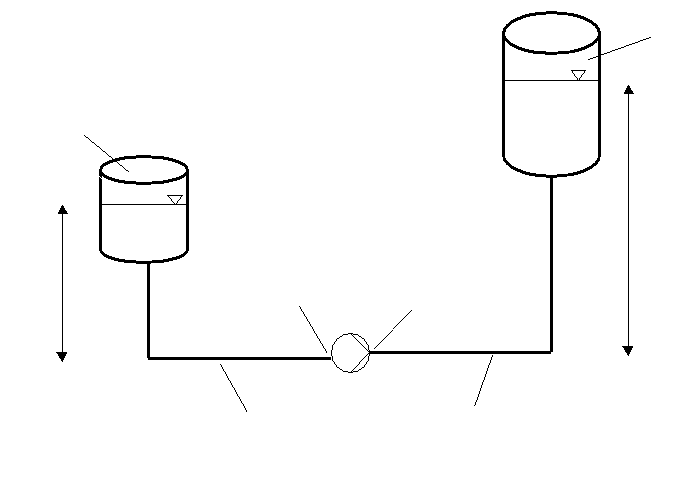 123
123- Suction vessel: establish pressure and the lowest relevant liquid level.
- Pump datum: define elevation and energy references unambiguously.
- Discharge vessel and piping: separate boundary conditions and losses.
Chapter 16RNET: manage topology and boundary conditions
RNET is registered for branched and meshed pipe networks. The network is built in a graphical editor; the chapter mask explicitly refers to the special menu. The reviewed source names “Rohrnetz” and “Netz einlesen”. The latter requests host-mediated import of old ROHRNETZ *.net files. If the graphical or import bridge is unavailable, the module reports that the corresponding route is unavailable in that environment.
In practice, a visible RNET row and licensed module name do not establish an operable network editor in every Web environment. No newly executed editor run is claimed here. Check the actual deployment. A missing editor cannot be replaced by manually entering a node count; the source receives V1/V2/V3 as header data from the network.
- Define nodes for connections and boundary conditions, branches for directed hydraulic sections, and a traceable elevation datum.
- Assign geometry, fluid state and included resistances to every branch. A direction sign is initially a calculation convention; a negative result may indicate actual flow in the opposite direction.
- Set sufficiently determined, consistent pressure and flow boundaries. Do not arbitrarily prescribe all node pressures and all branch flows simultaneously.
- After calculation, check mass balance at every node, energy consistency along paths and the pressure profile.
- Change one resistance or withdrawal deliberately and examine redistribution across the connected network.
Important connection limit: The reviewed RNET chapter code excludes conventional connections to other chapters. A conceptual flow of WTS → loss data → pipe network must therefore not be presented as an automatically available ordinary variable link. Transfer and modelling use the routes provided by the actual editor and require explicit acceptance checks.
Back to top ↑Chapter 17Check example: two parallel branches
Analytical network teaching example, not an RNET live case. Two horizontal parallel branches connect the same nodes A and B. Both use a fixed quadratic resistance relationship Δp = R·V̇². Resistances are R1 = 1,000,000 Pa/(m³/s)² and R2 = 4,000,000 Pa/(m³/s)². Total flow 0.030 m³/s and an arbitrary common pressure datum are prescribed; both branch flows and pressure difference are sought. There are no additional withdrawals or pumps within the branches.
Both branches have the same pressure difference. Thus R1·V̇1² = R2·V̇2² and, for positive flows, V̇1/V̇2 = √(R2/R1) = 2. Combining this with V̇1 + V̇2 = 0.030 m³/s gives V̇1 = 0.020 m³/s and V̇2 = 0.010 m³/s. Both yield Δp = 400 Pa. The solution requires two checks: node conservation and identical path difference.
If only R1 doubles to 2,000,000 while total flow remains fixed, the previous 2:1 split does not persist. The ratio drops to √2:1; flows become approximately 0.017574 and 0.012426 m³/s, with a common pressure difference of about 617.66 Pa. A local resistance increase therefore affects both branches. This is why independent pipe calculations with unchanged flows cannot replace a network assessment.
In real networks, resistances are often flow-dependent, pressure sources may be coupled and reverse flow may occur. Node and energy consistency still apply while the algebra becomes more demanding. For compressible networks, check mass flows at nodes; volume flows may be summed directly only at a common state reference.
Back to top ↑Chapter 18Connect WTS, properties and pressure loss
A defensible hydraulic heat-exchanger case starts with the corresponding thermal operating case. Transfer the tube side, fluid, mass flow, mean state, wall state and actual geometry unambiguously. The WTS tree may contain property child chapters; their presence alone does not establish that every required field is correctly transferred into a separately created RDV case.
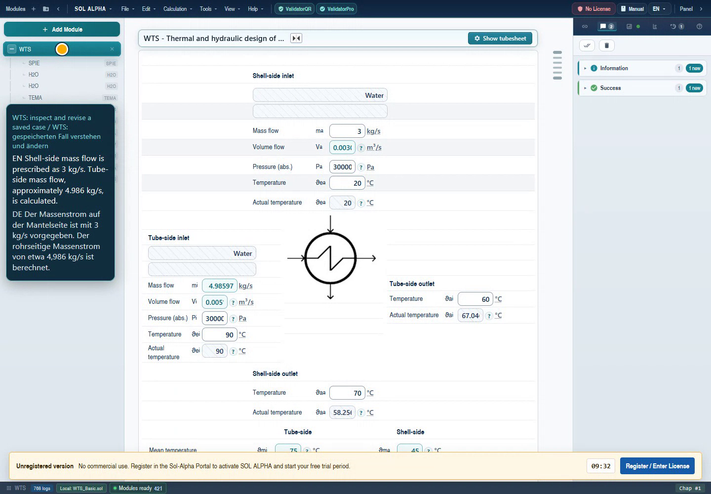 123
123- WTS distinguishes mass flow from actual volume flow.
- Pressure fields are explicitly labelled “Pressure (abs.)”.
- Inlet and outlet states belong to one case but different locations.
The genuine historical image shows the operating mask, not pressure-loss evaluation. Visible mass and volume flows belong to different states and sides. Absolute-pressure labelling matters for the connection; tightly displayed numbers are not transcribed here as exact hydraulic references. Visible messages and licence notices remain unchanged.
- Create a mapping table containing source chapter, source field, target chapter, target field, unit and state. Identify automatic transfer, explicit connection or manual transfer.
- For RDV, particularly review parallel-tube count, passes, mass flow and the distinction between fluid and wall properties.
- Make one small, physically acceptable source-input change. Check that the target recalculates and is not blocked by its own prescribed value.
- Restore the original value and compare inputs, results and connection status with the saved baseline.
- Transfer only the agreed complete component loss into the system budget. Do not double-count nozzles and pipe sections already included.
This is a prepared connection and roundtrip plan. No new RDV/NPSH/RNET connection run exists for this edition. The RNET special editor requires its own transfer routes; conventional chapter connections are explicitly restricted there.
Back to top ↑Chapter 19Pump curve, system curve and power
The steady operating point of a centrifugal pump is determined by the interaction of pump and system curves. The system contains static pressure/elevation contributions and flow-dependent losses. A pure loss curve through the origin therefore does not describe every system. At the considered flow, the pump must supply the required energy difference; the selected point must also lie within its suitable operating range.
The NPSH source describes a special menu for displaying pump and system curves. V41–50 hold volume-flow points and V51–60 their corresponding heads. These pairs belong to one manufacturer curve, speed and impeller configuration. Do not fill missing data with arbitrary smooth points. Check the actual graphical dialog and its availability in the deployed host; this edition contains no new curve screenshot.
For incompressible liquid, Phyd = ρgV̇H provides a useful energy check. Input power associated with pump efficiency follows as P = Phyd/η. Motor and drive losses may require further efficiencies depending on the system boundary. State whether “power” means hydraulic power, pump-shaft power or electrical input.
In the reviewed module, differential pressure V21 gives V22 through H = Δp/(ρg). For a complete independent energy balance, also review the definition of measurement sections and velocity contributions. Historical archive checks confirm this particular route, not every possible pump arrangement. The DOE pumping sourcebook provides engineering context for system, characteristic curve and energy consumption.
Back to top ↑Chapter 21Investigate implausible results systematically
| Observation | Check first | Engineering interpretation |
|---|---|---|
| Velocity far too high | m³/h versus m³/s; inside versus outside diameter; parallel count | A flow-unit error of 3,600 strongly affects Δp in a quadratic approximation. |
| Reynolds wrong by orders of magnitude | mPa·s versus Pa·s; μ versus ν | Start with the independent property relationship. |
| Friction factors differ by about four | Darcy/Fanning and the actual equation | Not automatic evidence of a defect. |
| RDV total loss too high | Nozzles counted twice; passes and parallel tubes | Check component groups and balance boundary. |
| Unexpectedly high NPSH | Absolute pressure in gauge field; atmosphere counted twice | Check V4/V11/V2 on one consistent reference. |
| Power Infinity or blank | Efficiency, input data and calculation status | V40 = 0 is not an acceptable power assumption. |
| Network mask has no entry fields | RNET special editor and host support | Header mask does not contain full topology. |
| Change does not reach target | Connection, independent prescription and calculation status | Check source and target values together with units. |
| Changed case jumps or stalls | Regime transition, conflicting inputs, missing properties | Isolate causes individually and retain the baseline. |
Start at the first implausible intermediate quantity. If velocity and Reynolds number agree, re-entering all data is rarely the best next step. Examine resistance modelling and summation specifically. If properties already disagree with the state, resolve that before assessing hydraulics.
A missing table dataset can affect a calculation route. For example, the RDV source contains a message and fallback value for a missing correction table. A displayed numerical result does not make the message irrelevant. Record such notices and check the data installation without removing documented warnings from images.
Back to top ↑Chapter 22Save, reopen and review the calculation
A traceable closeout consists of more than a PDF of final numbers. Save the native project or the dataset supported by the particular tool under a meaningful case identifier. Associate its property source, geometry revision, operating conditions and manufacturer curve. An exported report is a snapshot and does not necessarily contain all connections or the graphical network plan.
- Save the normal case after calculation and document prescribed values, free results and connections.
- Create a changed case with one clearly identified change and its own filename. Preserve the reference.
- Close and reopen an approved copy. Compare fluid, units, calculation direction, geometry and connection partners as well as final numbers.
- Make and reverse a small acceptable change. Check whether the original state and results return.
- For RNET, additionally review nodes, branches, boundaries and reconstruction of editor state. Give legacy *.net imports their own comparison report.
This is a concrete acceptance template; no new RDV, NPSH or RNET save/reopen run is evidenced for this edition. The historical NPSH file describes a regression test and is not a directly loadable SOL project. The bundled examples.json is also readable documentation, not a project archive.
Finally review pressure references, units, fluid state, regime, component summation, network balance, pump point and NPSH criterion. Record missing information together with its effect. “Calculation successful” is software status; compliance with process and manufacturer requirements requires separate judgement. Do not inherit case approval from historical test metadata.
Back to top ↑Chapter 23Look up fields and units
The table maps 106 specific identifiers. Read multiple identifiers in each row in the stated order. Display units may differ; this table gives module units from the reviewed definitions. Input, output or linked-target status depends on the selected calculation route. Internal helper fields and complete special-editor datasets are not presented as ordinary user inputs.
NPSH
| Field ID | Quantity | Module unit | Operating guidance |
|---|---|---|---|
| NPSH: V2 | Absolute vapour pressure | Pa | For the pumped fluid at operating temperature. |
| NPSH: V3 | Density | kg/m³ | Shared by pressure head, power and pipe flow. |
| NPSH: V4 / 14 | Suction/discharge vessel gauge pressure | Pa | Do not add barometric pressure again to these inputs. |
| NPSH: V5 | Approach velocity | m/s | Establish the energy reference point; not automatically equal to V29. |
| NPSH: V6 / 15 | Suction/discharge elevation | m | Use a consistent pump datum and signs. |
| NPSH: V7 / 16 | Suction/discharge pipe loss | Pa | Friction and fittings of the respective section. |
| NPSH: V8 / 11 | Altitude / barometric pressure | m / Pa | Source route relates altitude and atmospheric pressure; check alternative specification. |
| NPSH: V9 / 10 | Required / available NPSH | m | Compare manufacturer and system quantities at the same operating point. |
| NPSH: V12 / 13 | Pump description / fluid | − | Text fields, not numerical physical inputs. |
| NPSH: V17 / 18 | Elevation pressure terms | Pa | A negative historical suction term is consistent with positive flooded suction. |
| NPSH: V19 / 20 | Pump-nozzle pressures | Pa | Source equation includes barometric pressure: absolute values. |
| NPSH: V21 / 22 | Differential pressure / head | Pa / m | Source route H = Δp/(ρg); also review energy datum and velocities. |
| NPSH: V23 / 24 | Pump power / volume flow | W / m³/s | Power requires positive efficiency. |
| NPSH: V25 | Dynamic viscosity for pipe calculation | mPa·s | Source equation multiplies by 0.001 for SI Reynolds number. |
| NPSH: V26 / 32 | Pipe inside diameter | m | Suction and discharge respectively. |
| NPSH: V27 / 33 | Absolute roughness | m | Not relative roughness and not automatically millimetres. |
| NPSH: V28 / 34 | Pipe length | m | Actual section length; fittings separately. |
| NPSH: V29 / 35 | Pipe velocity | m/s | From actual volume flow and free pipe area. |
| NPSH: V30 / 36 | Pipe friction factor | − | Darcy convention in the reviewed NPSH source route. |
| NPSH: V31 / 37 | Reynolds number | − | Use matching dynamic viscosity and density. |
| NPSH: V38 / 39 | Fitting loss coefficient | − | Observe the reference diameter of the corresponding pipe. |
| NPSH: V40 | Pump efficiency | % | 75 means 75%; zero does not yield finite source-route power. |
| NPSH: V41 / 42 / 43 / 44 / 45 / 46 / 47 / 48 / 49 / 50 | Curve volume-flow points | m³/s | Use in pairs with V51–60; no arbitrary curve points. |
| NPSH: V51 / 52 / 53 / 54 / 55 / 56 / 57 / 58 / 59 / 60 | Curve head points | m | For the reviewed speed and impeller geometry. |
RDV
| Field ID | Quantity | Module unit | Operating guidance |
|---|---|---|---|
| RDV: V1 / 2 | Mean fluid/wall temperature | °C | Different states for corrections. |
| RDV: V3 / 4 | Mean / wall-state density | kg/m³ | Do not mix arbitrary fluids. |
| RDV: V5 / 6 | Heat capacities | J/(kg·K) | Fluid and wall states of the same stream. |
| RDV: V7 / 8 | Thermal conductivities | W/(m·K) | Property, not a heat-transfer coefficient. |
| RDV: V9 / 10 | Dynamic viscosities | mPa·s | Viscosity ratio affects the friction correction. |
| RDV: V11 / 12 | Nozzle inside diameters | m | Inlet and outlet separately. |
| RDV: V13 / 14 | Passes / parallel tubes | − | Distinguish tubes in parallel per flow path from total tubes. |
| RDV: V15 / 16 | Tube length / inside diameter | m | Friction path and free area. |
| RDV: V17 / 18 | Outside diameter / wall thickness | m | Geometrically consistent with inside diameter. |
| RDV: V19 / 53 | Mass flow / volume flow | kg/s / m³/s | V̇ = ṁ/ρ at the corresponding mean state. |
| RDV: V21 / 22 | Tube velocity / Reynolds number | m/s / − | First hydraulic plausibility check. |
| RDV: V25 / 26 | Turn coefficient / isothermal friction factor | − | V26 follows Fanning convention, not NPSH Darcy. |
| RDV: V27 / 28 / 29 | Corrections / resulting friction factor | − | V29 = V26 · V27 · V28 in the reviewed source route. |
| RDV: V30 / 31 / 32 | Nozzle / entry-exit / tube friction | Pa | Separate loss groups before checking the total. |
| RDV: V33 / 34 | Fouling multiplier / total loss | − / Pa | Total = V30 + V31 + V33 · V32. |
| RDV: V36 / 43 | Construction / phase | − | Straight=1, U=2, bends=3; liquid=0, gaseous=1. |
| RDV: V44 / 45 / 48 | Inlet/outlet temperature / inlet pressure | °C / °C / Pa | State data for the operating case; establish the pressure reference. |
| RDV: V46 / 47 / 49 / 50 | Nozzle velocities / densities | m/s / m/s / kg/m³ / kg/m³ | Evaluate inlet and outlet conditions separately. |
| RDV: V51 / 52 | Inlet/outlet nozzle loss | Pa | Do not add subresults again to an already complete total. |
RNET
| Field ID | Quantity | Module unit | Operating guidance |
|---|---|---|---|
| RNET: V1 / 2 | Node/branch count | − | Feedback from the network editor, not a substitute for topology. |
| RNET: V3 | Fluid selection | − | Selection reported by the graphical host. |
| RNET: V10 | Comment | − | Case description; not a hydraulic boundary condition. |
Chapter 2420 frequently asked practical questions
Which module should I start with?
Choose by task: RDV for a heat-exchanger tube side, NPSH for a liquid-pump system, RNET for the coupled network. FDP, DROS, CAV and other members each address separate models.
Is pressure loss always the measured pressure difference?
No. Velocity and elevation may change between measurement locations. Read static pressure difference with its energy balance; irreversible losses form a distinct contribution.
Why do two modules show different friction factors?
First check convention. Darcy is four times Fanning. The reviewed NPSH and RDV routes use different definitions; RDV also contains thermal corrections.
Can I insert μ in mPa·s directly into the SI Reynolds equation?
No. Multiply the numerical value by 0.001 to obtain Pa·s. Also distinguish dynamic viscosity from ν in m²/s.
Why is nominal pipe size insufficient?
Flow area depends on actual inside diameter. Wall thickness, pipe schedule, lining and deposits can change it. Record the source of the inside diameter used.
Are more passes in RDV always better?
More passes change parallel flow area, path length and turning losses. Assess thermal benefit and hydraulic cost together. There is no universal direction of improvement.
Why does RDV need wall-state properties?
The source route accounts for viscosity ratio and convection effects. These are properties of the same fluid at the wall state, not an arbitrary second substance.
What does fouling multiplier V33 mean?
In the reviewed RDV total it multiplies tube-friction loss. It is a hydraulic multiplier and is not automatically identical to a thermal fouling resistance in m²K/W.
Should I add V51/V52 again to the RDV total?
Not without checking. They are nozzle subresults; the total already contains its intended nozzle contribution. Trace the balance boundary and actual summation route.
Is NPSH V4 absolute pressure?
In the reviewed module it is vessel gauge pressure. The source adds barometric pressure V11. An already absolute value in V4 therefore gives the wrong pressure level.
Does high NPSH mean high pump head?
No. NPSH describes suction-state margin above vapour pressure on a defined reference. Head describes pumping duty. The historical case shows high available NPSH with low head.
Is NPSHA equal to NPSH3 sufficient?
That is not general acceptance. NPSH3 refers to a 3% head drop. Define the required cavitation criterion and margin for the pump and application.
Why does the historical archive contain Infinity?
It prescribes efficiency of 0%. The power formula divides by this value. An expected infinite result and expectSuccess=true do not make it a valid pump design.
Can I cite the 75%-efficiency power as a measured Web result?
No. It is an explicitly separate analytical change to historical hydraulic quantities. No new module entry, run or reopening evidence was produced for it.
Why does warmer fluid not automatically improve NPSH?
Lower viscosity can reduce losses while vapour pressure increases. Assess all consistent properties and the operating point that actually governs.
Where do I enter the network in RNET?
The reviewed route uses the graphical “Rohrnetz” special menu. The ordinary mask is not a substitute. Editor and legacy-file import availability depend on the actual host.
Can RNET use conventional WTS chapter links?
The reviewed chapter code excludes ordinary connections. A conceptual relationship remains possible but must use and verify the editor and transfer routes actually provided.
Should I add parallel-branch losses?
Branches between the same nodes have compatible energy differences and split flow accordingly. Their losses are not added as if the resistances were in series.
Is orifice metering differential pressure the permanent loss?
Not generally. Measurement locations, pressure recovery and geometry matter. Use the quantity defined by the specific DROS/RO route for metering or the system loss budget.
Does this package complete every individual module manual?
The package map is complete and RDV/NPSH/RNET are detailed teaching routes. Standalone full manuals for all variants and fresh live, connection and reopening evidence remain separate work items.
Back to top ↑Chapter 25Compact glossary and transfer checklist
| Term | Meaning in the workflow |
|---|---|
| Actual volume flow | Volume per unit time at the specified local state. |
| Standard volume flow | Volume flow referenced to an explicitly specified standard state. |
| Dynamic pressure | ρv²/2; reference for many loss coefficients. |
| Loss head | Irreversible loss as energy per unit weight, ΔpL/(ρg). |
| Darcy factor | Pipe-friction definition λD; four times the Fanning factor. |
| Fanning factor | Friction definition fF; retain its equation convention. |
| Absolute roughness | Length representing modelled wall roughness; distinguish from ε/D. |
| Zeta coefficient | Local loss coefficient with a defined reference velocity. |
| Pump head | Pump-specific energy with a defined balance boundary. |
| NPSHA | NPSH supplied by the system at the defined reference. |
| NPSHR / NPSH3 | Pump requirement with cavitation criterion; NPSH3 is the 3% case. |
| Node balance | Steady mass flows at a node sum to zero. |
| Boundary condition | Prescribed pressure, addition/withdrawal or another model input. |
| Inverse calculation | Change of sought quantity with a consistent known-value set. |
| Roundtrip | Change and restoration, or saving and reopening, with comparison. |
When handing over a loss value, identify at least the component/section, fluid and state, flow, pressure reference, included subcomponents, geometry revision and calculation source. A pump also requires its curve, speed, efficiency definition and NPSH criterion. A network additionally requires topology and boundary conditions.
Technical package membership and engineering tasks can overlap. WTS and property modules therefore appear as neighbouring workflows without altering membership in the complete 24-member group listed here. An explanation in a package overview does not automatically complete a standalone module handbook.
Back to top ↑Chapter 26Sources, image provenance and reviewed scope
Web source revision: main13.0 / 1cd12e8b173ba72aa5c95c98a14772b7ee537997. All-Dev revision: fix-iteration/v10 / 40606b705b2df95e550ffef5e98ab733ccc66229. The source inventory contains package configuration, registered descriptions and hashes of the RDV/NPSH/RNET definitions, masks and selected calculation routes actually examined. Recorded working-tree status distinguishes commit from local file state.
The example data contain an unaltered selection from the historical NPSH regression case of 29 April 2026, including original path, date, SHA-256 and actual archived expectations. Non-finite power remains visible. A clearly identified analytical pipe exercise is added. JavaScript checks independently evaluate its algebra; they execute no SOL plugins. Plugin build, a fresh live run, comprehensive Desktop/Web parity and new connection/reopening evidence are not documented.
Primary engineering references
- U.S. Department of Energy: Improving Pumping System Performance – relationship between system, pump curve, operating point and energy demand.
- KSB Centrifugal Pump Lexicon: NPSH – system quantity, pump requirement and different cavitation criteria, particularly NPSH3. No universal margin is inferred from this overview.
- NASA/CR—2007-215006 – definitions of Darcy and Fanning friction factors. Their module assignment is also established from the modules' own equations.
Images and limits
Image provenance documents unchanged original bytes. One approved historical WTS frame shows only the relevant operating-data context. An existing NPSH module drawing is identified as an illustration; its original creation date and author are not recorded. New numbering is separate HTML over the originals. Neither image shows a new RDV, NPSH or RNET run.
All 24 configured members are placed in context. RDV, NPSH and RNET are the detailed teaching routes; standalone full handbooks for every member and variant are not thereby complete. The manifest records the published scope. Text, images, search, print and language inheritance work locally; only further Internet sources require a connection.
Back to top ↑