Process & thermodynamics – Mass and energy balance calculations
Understand balance boundaries and fluid states, mix moist air correctly and connect process modules traceably.
No chapter found. Try another search term.
Chapter 01Understand process calculations as one connected task
This handbook connects mass and energy balances with modules that turn them into actual states and equipment requirements. A balance can close numerically while describing the wrong process: the reference mass may be wrong, a phase change omitted, temperatures reversed or a saved mixture curve associated with a different pressure. Work therefore begins with the model before filling in the mask.
The map covers all 15 configured members. BIL explains a heat-exchanger balance, PSYC interprets wet- and dry-bulb readings, MIFL mixes moist air, JTHO addresses natural-gas throttling, and NETZ connects multiple units in a steady system. Combustion, condensation, air cooling and time-dependent processes extend this context.
A useful reading order
For a heat exchanger, start with BIL and the numerical example. For air states, follow humidity terminology, PSYC and MIFL. For gas-pressure changes, read JTHO before transferring temperatures. A complete network also requires topology and boundary conditions.
This edition includes historical PSYC and JTHO regression values with provenance and hashes, new analytical exercises and operating workflows prepared from sources. Historical values were not newly executed in SOL here. Two genuine WTS images show process context; they are not presented as new standalone-module captures. Each case states its evidence level and outstanding execution evidence.
Back to top ↑Chapter 02Define the balance boundary and calculation direction first
Draw the installation as material streams and balance volumes. Mark inlets/outlets, heat input/output, mechanical work and possible accumulation. A steady balance assumes no relevant mass or energy accumulates in the control volume over the period considered. TIME instead addresses that accumulation and requires an initial state.
- Name the case and its task: required cooling flow, mixed temperature, air humidity or temperature after pressure reduction.
- Define substances, composition, phase, pressure reference and state locations. State whether a stream is referenced to dry air, moist air, fuel or total mixture.
- Specify exactly which quantity is sought. An inverse calculation replaces a former prescribed value with a target; it does not merely add another fixed boundary.
- Check property provenance and enthalpy references. Combine data from different sources only where their definitions are compatible.
- Calculate the simplest consistent case first. Check balance closure and intermediate results before linking further modules.
- Change one parameter deliberately, compare the effect and save both cases with their input status.
A result field can be stale despite displaying a number. Wait for completed calculation status and review messages. If another chapter prescribes a target, a local input can overconstrain the task or block the intended change. Record each value's role: prescribed, calculated or linked.
A short stream table supports reviewable transfer: identifier, from/to, fluid, composition, mass basis, flow, T, p and h. Do not fill missing engineering data with arbitrary default numbers.
Conceptual workflow diagram. Every actual automatic or manual data route is checked separately.
Back to top ↑Chapter 03Understand the 15 package modules
The following list fully represents configured membership. It is an engineering selection aid, not evidence of a particular licence or currently running module. BIL, PSYC, MIFL, JTHO and NETZ form the detailed workflows; other members are placed in context by task and essential transfer data.
| Module | Task | Selection guidance and limits |
|---|---|---|
| ABGV | Flue-gas losses | Combine measured gas fractions, temperature, air humidity and fuel basis. Establish dry/wet reference basis and heating-value units before evaluating losses. |
| BIL | Heat-exchanger material and heat balance | Relate inside/outside streams, duty, temperature difference, heat transfer and area. Detailed teaching route; not an arbitrary reaction or flowsheet solver. |
| FLAM | Combustion-chamber calculation | Combustion-chamber task with appropriate fuel and heat-transfer description. Check actual mask and model scope before use; the registry provides no detailed method claim. |
| FN | Corrected temperature difference | Actual log-mean temperature difference for appropriate exchanger arrangements. Establish configuration and temperature references; a correction factor is not an arbitrary margin. |
| JTHO | Adiabatic natural-gas throttling | Isenthalpic state change using natural gas H/L or an appropriate custom composition. Distinguish forward and inverse direction through the prescribed temperature/pressure values. |
| MIFL | Mix two moist-air streams | Balance dry air, water and enthalpy together. Distinguish total moist-air flow from dry-air basis; check possible condensation in the mixed state. |
| PSYC | Evaluate an aspiration psychrometer | Convert wet-/dry-bulb temperatures and total pressure into an air state. Two thermometer columns are not two independent process streams. |
| RG | Flue-gas properties | For solid fuels, fuel oils and gases in the appropriate fuel model. Document composition, combustion-air basis and reference state together. |
| TIME | Transient heating and cooling | Time-dependent temperature change for supported tasks. Initial state, heat capacity and boundary conditions are required in addition to the steady end state. |
| KOKU | Mixture condensation curve | Calculate a curve between inlet/outlet or enter suitable data manually. Saved curves retain composition, pressure and data revision as validity context. |
| KONR | Condenser area and tube count | Relate cooling-water flow, tube geometry and heat load for condenser sizing. Water state and allowable temperature rise must belong to the same load case. |
| KPRE | Marginal cooling-water price | Compare dry/wet cooling using costs, annuity, annual utilization and evaporation. Historical inputs are not current price recommendations. |
| PLRE | Hot-air recirculation at an air cooler | Assess performance loss from recirculated warm air with the appropriate installation and air guidance. Local inlet temperature may differ from ambient. |
| RKS | Multicomponent phase equilibrium | RKS equation of state with selected components and consistent composition. Component identity, mole/mass basis and model range determine the result. |
| NETZ | Steady heat-exchanger and plant network | Graphical NETZ.Plan and stationary SOLVNET route with modules such as WTS/AC. Process networks and hydraulic RNET are different tasks and data routes. |
A package overview does not complete standalone full manuals for every variant. Manufacturer data, historical property files, special editors and code-related boundary conditions require additional identification in the actual project.
Back to top ↑Chapter 04Enthalpy, power, signs and reference mass
Enthalpy is a state property. For steady flow without relevant changes in kinetic or potential energy, ṁ·Δh is the corresponding energy-change rate. Specific enthalpy in J/kg becomes unambiguous only when the kilogram is defined. For water it may mean one kilogram of total substance; for moist air it often means one kilogram of dry air. An identical unit symbol does not remove this difference.
Q̇ = ṁ (hout − hin) · for justified constant cp: Q̇ = ṁ cp(Tout − Tin)
With this stream convention, heating is positive and cooling negative. In an externally adiabatic heat exchanger, the signed changes of both streams must cancel. A positive transferred duty is often expressed as a magnitude; do not insert that magnitude into a signed balance without explanation.
The reviewed BIL source uses V13 + V14 = V15. V15 is labelled heat loss, but its algebraic definition matters. Do not use a positive number merely because “loss” intuitively sounds positive. The normal example uses V15 = 0; for an actual environmental loss, reconcile the intended direction with this module equation.
Watts measure power; joules measure energy. 1 kW = 1,000 W and 1 kWh = 3.6 MJ. Stored thermal energy requires time integration of power. When cp varies or phase changes occur, an enthalpy difference is the appropriate starting point. Arbitrarily increasing heat capacity replaces neither a condensation curve nor latent heat.
Back to top ↑Chapter 05BIL: assign the two streams and heat exchanger
In the reviewed version, BIL is a material and heat-balance module for the inside and outside streams of a heat exchanger. It includes film coefficients, wall, area and geometry data. It therefore extends beyond a single Q̇ equation but is not a general reaction or plant-flowsheet solver. “Inside” and “outside” identify geometry; they do not automatically mean “hot” and “cold”.
- Assign both fluids to the correct sides. Specify their states and suitable density/heat capacity or review transfer from connected modules.
- Select arrangement V26: counterflow 1, parallel flow 2 or crossflow 3. Geometry V51 distinguishes the documented tube route from other geometry approaches.
- Prescribe a sufficient combination of mass flows and inlet/outlet temperatures. Leave the sought temperature or flow free.
- First check signed duties V13/V14 and balance term V15.
- Then add suitable film coefficients, wall data and fouling resistance for overall k, required area and actual geometry.
Mean calculation temperatures V29/V30 and area margin V48 are locked in the reviewed initialization route and treated as derived quantities. Old fields V27/V28 participate in migration of former arrangement flags. They are not recommended here as modern ordinary selection controls. Use the actual selection in the current mask.
Required area V21 and actual area V47 are different quantities. Source-route margin V48 is (V47/V21 − 1)·100%. A negative result means actual area is below required area according to the selected model. Closing both stream balances does not make this deficiency disappear.
Back to top ↑Chapter 06Review temperature difference, correction factor and area
Heat transfer requires a driving temperature difference along the unit. Four terminal temperatures give a log-mean temperature difference according to the arrangement. Counterflow and parallel flow pair the temperatures differently. A list of four temperatures is therefore insufficient without flow direction.
ΔTlm = (ΔT1 − ΔT2)/ln(ΔT1/ΔT2) · Q̇ = k A ΔTeff
For equal positive terminal differences, the limit is exactly that common difference; direct substitution formally gives 0/0, which is not a physical impossibility. Opposite signs instead require review of arrangement, temperature assignment and physical feasibility. An arbitrary absolute value does not repair an incorrect process case.
In the documented crossflow route, BIL applies an available FN factor. FN addresses suitable exchanger arrangements. Transfer the factor together with its geometry and temperature definition. Check whether a temperature difference is already corrected before multiplying by FN again. The resulting area is only as defensible as k, the driving difference and their shared area reference.
For tube geometry, overall heat transfer includes inside/outside area conversion and wall resistance. Inside-area coefficients therefore cannot be compared indiscriminately with outside areas. Fouling in m²·K/W is a thermal resistance; a hydraulic fouling multiplier in a pressure-loss module means something different. See the DOE heat-transfer reference for engineering foundations.
Back to top ↑Chapter 07Place phase changes and mixture curves in context
Evaporation and condensation change enthalpy, often without a correspondingly large temperature change. A pure fluid at approximately constant pressure may transfer substantial heat at nearly constant saturation temperature. Multicomponent condensation often spans a temperature range with changing phase compositions. One mean temperature cannot fully represent that task.
BIL includes latent enthalpies and phase fractions for its intended routes. Do not add them to latent heat already fully represented by Δh. Decide whether sensible and latent contributions are balanced separately or through one consistent overall enthalpy difference. Double counting can create an apparently well-closed but incorrect heat-duty case.
RKS is registered for multicomponent phase equilibrium using the Redlich-Kwong-Soave equation. KOKU describes condensation curves between inlet/outlet states and, according to its registration, also permits manually entered curves. Saved curves belong to a composition, pressure and data revision. Renaming a curve at a different pressure does not make it suitable.
JTHO handles isenthalpic throttling with its own state check. The examined source aborts when gas/liquid two-phase conditions are detected before or after the throttle. Such a message is therefore not a direction to continue with averaged gas properties. Establish the appropriate phase-equilibrium or process route separately.
A curve transferred to a heat exchanger needs at least axis definitions, units, mass basis, pressure, composition, inlet/outlet and interpolation range. A saved filename alone does not document that meaning.
Back to top ↑Chapter 08Moist air: separate three easily confused quantities
Relative humidity φ describes water-vapour partial pressure relative to saturation pressure at the same temperature in the relationship used here. Humidity ratio x is water per mass of dry air. Degree of saturation ψ is x/xs. All three describe moisture but are numerically different. Relative humidity of 60% must not be entered as x = 0.60 kg/kg.
φ = pw/ps · x = (Ra/Rw) pw/(p − pw) · ψ = x/xs
A percentage display multiplies φ by 100. Total pressure p is absolute; water-vapour partial pressure pw is only its water contribution. At identical temperature and relative humidity, changing total pressure can change humidity ratio. A moist-air state therefore needs more than temperature and an unspecified “humidity value”.
PSYC processes wet- and dry-bulb readings from an aspiration psychrometer. The wet side is the saturated reference state used by its calculation route; the dry side describes the sought air state. The columns are not independent inlet and outlet streams. Actual measurement method, adequate aspiration and correct thermometer assignment are part of input quality; an arbitrary surface sensor does not provide a wet-bulb temperature.
Enthalpy h and specific volume v are expressed per kg dry air in the reviewed PSYC route. Moist-air density is therefore ρmoist = (1+x)/v. The reciprocal 1/v alone uses a different reference mass. The NBS/NIST psychrometric reference supports these distinctions; identical implementation of its complete models is not claimed.
Back to top ↑Chapter 09MIFL: balance water, dry air and energy together
MIFL mixes two moist-air streams and reports the mixed state and possible condensation. Begin with two fully defined air states and their mass flows. Temperature and relative humidity alone do not define an enthalpy flow; pressure and mass basis are also needed.
- Assign streams 1 and 2 to the actual inlet ducts. Establish temperature, total pressure and the appropriate humidity parameter.
- Decide whether known flow means moist air or dry air. Use V30/V31 or V33/V34 accordingly.
- Check x, h and the conversion ṁmoist = ṁdry(1+x) where that relationship describes the mixture.
- After calculation, review total dry-air flow V35, mixed humidity ratio V26, mixed enthalpy V50 and temperature V8.
- Check whether the mixed state contains liquid and read condensed-water flow V54 in kg/s.
The source route weights enthalpies with dry-air mass flows. Using total moist-air flows directly as weights without their respective moisture content generally gives a different balance. Relative humidities are not averaged arithmetically; a linear temperature average at different humidities is also valid only under justified additional assumptions.
The source contains separate routes for unsaturated states and states containing condensate. Humidity ratio on a total-water basis can therefore exceed saturation humidity ratio while the excess is treated as liquid. State whether condensate remains in the control volume or is subsequently drained. Do not automatically assign the total water loading, including separated liquid, to a downstream gas stream.
Back to top ↑Chapter 10First example: close a sensible-heat balance
Fully defined analytical teaching calculation, not a BIL live demonstration. Two liquid streams exchange heat in counterflow. Both use constant cp = 4,200 J/(kg·K) for this exercise. The exchanger is externally adiabatic; phase change and mechanical work are excluded. Values are teaching inputs, not newly calculated properties of a particular fluid.
| BIL mapping | Specified value | Status |
|---|---|---|
| V1 inside | 2.0 kg/s | Fixed |
| V2 outside | 3.0 kg/s | Fixed |
| V7/V8 | 4,200 J/(kg·K) | Fixed |
| V9/V10 inside | 90 / 60 °C | Fixed |
| V11 outside | 20 °C | Fixed |
| V12 outside | Sought outlet temperature | Free |
| V15 loss term | 0 W | Fixed |
| V26 | 1, counterflow | Fixed |
| V33–36 | No latent heat; phase remains liquid | Phase route inactive or appropriately zero |
| V13/V14 | Heat duties | Results |
The inside stream cools: Q̇i = 2·4,200·(60−90) = −252,000 W. The outside stream receives +252,000 W. Its temperature therefore rises by 252,000/(3·4,200) = 20 K, giving an outlet of 40 °C. The balance sum is zero. An outlet of −40 °C or an also-negative outside duty would not be an acceptable alternative sign convention; it would require an assignment check.
Counterflow terminal differences are 90−40 = 50 K and 60−20 = 40 K. Thus ΔTlm = 44.8142 K. If an additionally justified overall coefficient k = 1,000 W/(m²·K) is prescribed on the agreed area basis, the area exercise gives A = 5.62322 m². That k is an additional teaching assumption; it was not derived from tube geometry or actual film coefficients.
In a later isolated BIL run, review every known/free state and the additional inputs actually required. A stream balance can be fully determined before the complete geometry evaluation. Do not expect every mask to produce a complete equipment result without all model-dependent data.
Back to top ↑Chapter 11Change and inverse calculations with a clear direction
More hot flow with the same required cooling
In the analytical BIL case, only V1 increases from 2.0 to 2.4 kg/s. The hot outlet deliberately remains prescribed at 60 °C; the cold stream remains 3.0 kg/s at 20 °C inlet. Duty is now 302.4 kW and the calculated cold outlet becomes 44 °C. Terminal differences become 46 and 40 K; ΔTlm = 42.9301 K. Retaining assumed k = 1,000 gives a new required area of 7.04400 m².
This explicitly calculates a changed design requirement. Existing area of 5.62322 m² does not grow as a result. Rating the same actual exchanger instead requires retaining its area and releasing an appropriate outlet state. This distinction is central to operation: which temperature is a required prescribed value and which is the outcome of existing geometry?
Find cooling flow for a 50 °C outlet
Return to the original hot stream and its 252 kW cooling duty. The cold stream must now heat from 20 to 50 °C. Prescribe V12 = 50 °C and release V2. The analytical inverse calculation gives ṁcold = 252,000/(4,200·30) = 2.0 kg/s. Insert this flow back into the forward balance; it must close at 50 °C.
These numbers are independently calculated teaching values, not a newly executed BIL inverse run. In the module, additionally check whether a link still fixes V2 and whether cp, phase and geometry suit the changed case. After every change, assess thermal duty, area and hydraulic limits together.
Back to top ↑Chapter 12Historical PSYC case: read wet and dry correctly
Historical regression reference dated 6 May 2026, not newly executed. Prescribed values are wet-bulb V6 = 50 °C, dry-bulb V7 = 60 °C and total pressure V8 = 100,000 Pa absolute; the archive records design type 1. Their order is established from actual mask labels and source equations. The 50 °C value is not a dew point and the temperatures are not heat-exchanger inlet/outlet temperatures.
For a prepared replay, prescribe only these physical drivers and calculate the corresponding air state. The archive contains many expected helpers and model constants, including specific gas constants and heat capacities. They are not taught here as additional measured values to fix manually. The source relates the second pressure column to the first.
| Field | Result | Archived value | Unit |
|---|---|---|---|
| V11 | Air relative humidity | 58.918583 | % |
| V18 | Saturation pressure at wet-bulb temperature | 12344.605 | Pa |
| V19 | Saturation pressure at dry-bulb temperature | 19933.037 | Pa |
| V21 | Air water-vapour partial pressure | 11744.263 | Pa |
| V23 | Air humidity ratio | 0.082772695 | kg/kg trocken / dry |
| V25 | Saturation humidity ratio at dry-bulb temperature | 0.1549089 | kg/kg trocken / dry |
| V27 | Air degree of saturation | 0.53433144 | − |
| V29 | Air enthalpy | 276541.62 | J/kg trocken / dry |
| V31 | Air specific volume | 1.0833749 | m³/kg trocken / dry |
| V33 | Moist-air density | 0.9994442 | kg/m³ |
Relative humidity is approximately 58.919% and humidity ratio approximately 0.082773 kg water per kg dry air. These describe the same state using different definitions. Degree of saturation is about 0.53433, again different from relative humidity as a decimal. The wet reference column has 100% relative humidity in the model; that does not make the actual air saturated.
The example file preserves original date, inputs, expectations, units and SHA-256. The original plugin build is not independently documented. These values are therefore historical regression expectations with specific provenance, not a general accuracy guarantee for the instrument or current module version.
Back to top ↑Chapter 13Check PSYC results with three relationships
Historical results can be checked for internal consistency without reimplementing the complete property model. The checks below use archived saturation pressures and model constants. They confirm relationships within the stored case; they do not measure a current SOL execution or replace independent reference measurement.
- Partial pressure: pw = φ·ps, with φ as a fraction. Combining 58.918583% and 19,933.037 Pa gives approximately 11,744.263 Pa.
- Enthalpy: The documented model h = 1,004·t + x·(2,501,600 + 1,860·t), with t = 60 °C and x = 0.082772695, gives about 276,541.62 J/kg dry air.
- Density: With v = 1.0833749 m³/kg dry air, (1+x)/v = 0.9994442 kg/m³ moist air. The reciprocal 1/v alone uses a different mass basis.
Rounding of archived individual values produces small residual differences. Documentation tests set explicit tolerances for this algebra. Archive tolerance 0.01 is not automatically translated as “1% model accuracy”. Measured temperature uncertainty and model uncertainty are also separate contributions.
Prepare a change and return
A later live comparison can use a slightly changed wet-bulb reading at the same total pressure while retaining dry-bulb temperature. Observe φ, x and h together. Simply swapping the thermometer values is not a meaningful changed case. Restore the initial value and check original inputs and outputs. Before an inverse calculation, establish which input combinations the actual module version supports; arbitrary reversal of every helper field is not promised here.
Back to top ↑Chapter 14Teaching example: mix two air streams on a dry-air basis
Analytical MIFL check calculation, not a new module run. Two steady air streams mix without external heat at common total pressure of 100,000 Pa. Stream 1 has 30 °C, x1 = 0.010 kg/kg dry and 2.0 kg/s dry air. Stream 2 has 10 °C, x2 = 0.004 kg/kg dry and 1.0 kg/s dry air. Teaching algebra uses constant cp,a = 1,004 and cp,v = 1,860 J/(kg·K), and hv,0 = 2,501,600 J/kg. The mixed state is treated as unsaturated; verify this in a module execution.
Dry-air flows sum to 3 kg/s. Water balance gives xM = (2·0.010 + 1·0.004)/3 = 0.008 kg/kg dry. The stated enthalpy model yields h1 = 55,694 J/kg dry and h2 = 20,120.8 J/kg dry. Weighted mixed enthalpy is hM = 43,836.2667 J/kg dry. Rearranging the same model gives TM = 23.38201 °C.
Moist inlet mass flows are 2.020 and 1.004 kg/s, totalling 3.024 kg/s. These are not the weights for the dry-air-based enthalpies above. Averaging 30 and 10 °C with arbitrary total-mass weights or arithmetically mixing 50%/80% relative humidity would use a different balance.
As an isolated change, double only dry-air stream 2 to 2 kg/s. Then xM = 0.007 kg/kg dry and the same algebra gives TM = 20.05487 °C. Temperature is near 20 °C but, because water loading differs, not exactly the simple average. Update complete mixed properties and the phase check before transfer to a cooler or condenser.
Back to top ↑Chapter 15JTHO: recognize an actual historical inverse case
Historical JTHO reference dated 27 June 2026; not newly executed. The case selects natural gas L with V20 = 2. Prescribed values are upstream pressure V4 = 200,000 Pa absolute, downstream pressure V5 = 100,000 Pa absolute and temperature after the throttle V3 = 50 °C. The sought and archived expected temperature before the throttle is V2 = 50.36315 °C. Registration often describes the forward task; this particular dataset is explicitly inverse.
| Component | Archived mole percentage |
|---|---|
| N2 | 12.6 mol-% |
| CH4 | 82.0 mol-% |
| CO2 | 1.2 mol-% |
| C2H6 | 3.3 mol-% |
| C3H8 | 0.6 mol-% |
| C4H10 | 0.3 mol-% |
| H2, pentane, hexane | 0 in the documented prescribed/result state |
The six positive fractions sum to 100 mol-%. They are not mass percentages. The model represents adiabatic throttling with no relevant external work or kinetic/potential-energy change as an isenthalpic process. “Adiabatic” does not generally mean “isentropic”. A pressure reduction therefore does not imply the temperature change of an idealized turbine expansion.
The stored states give a temperature drop of approximately 0.36315 K. This is not used to infer one universal constant Joule-Thomson coefficient for all natural gases and pressure intervals. Composition and state affect the path. The source checks potential two-phase conditions and contains an associated abort message.
Prepare a forward check
A new isolated check would prescribe V2 at the archived upstream value, release V3 and retain both pressures and composition. It would be expected to return near 50 °C within the actual model and documented tolerance. That roundtrip was not executed here. The source also distinguishes Pa from internal bar; transfer pressures only with explicit units.
Back to top ↑Chapter 16NETZ: build a traceable steady process network
NETZ connects heat exchangers and plant units in a steady network. Registration and source route use the graphical NETZ.Plan editor and SOLVNET calculation. The task concerns streams, temperatures, equipment coupling and network heat exchange. Hydraulic pipe-network module RNET in the pressure-loss package addresses a different task. Similar names do not imply interchangeable project files or identical boundaries.
The examined NETZ.Plan interaction contains nodes, directed links, mass flows, inlet temperatures and paired tube/shell sides of heat exchangers. Each exchanger pair has a common group assignment. Placing two symbols close together does not replace that assignment. The actual editor is provided by the host; source code or an archived mask is not evidence of a currently available live dialog.
- Define inlet streams with fluid, flow and state, plus outlets and any recycles.
- Pair both sides of every heat exchanger and connect their stream paths in the correct direction.
- Check mass sums at splits and mixing points. Temperature sums alone are not an energy balance.
- Add only appropriate equipment data, for example from the corresponding WTS or AC case, and identify their calculation revision.
- After the steady run, review global energy conservation, outlet temperatures, directions and local equipment conditions.
A numerical iteration limit is not a physical accuracy requirement. A converged calculation can use incorrect topology; arbitrarily increasing iterations does not make a nonconvergent recycle case physically correct. Start with a clear open network and add recycles gradually. No newly executed NETZ.Plan or save run exists for this edition.
Back to top ↑Chapter 17From the balance to WTS equipment and back
A heat balance supplies the required duty, while actual equipment geometry determines which states can be achieved under specified conditions. WTS distinguishes these in its operating context. Transfer more than one duty number from a balance: include both fluids, flows, temperature targets, pressure states and the appropriate calculation direction.
 123
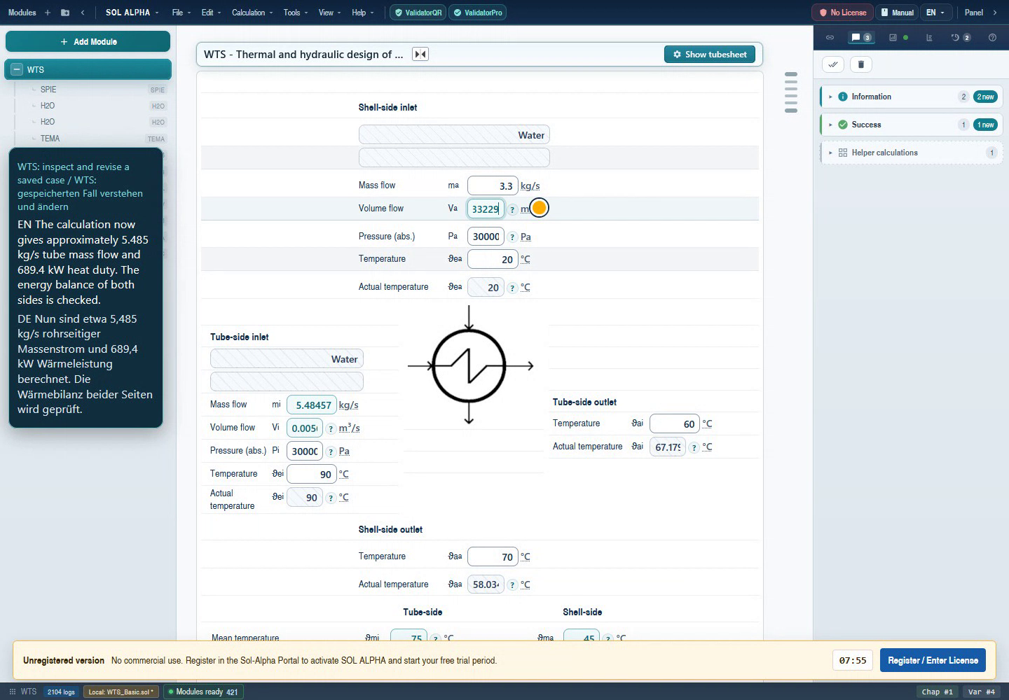
123Unmodified frame from the approved WTS video of 6 September 2026 at 225 s. Shows WTS context, not a newly captured BIL/PSYC/MIFL/JTHO/NETZ mask. Visible notices and display limitations remain unchanged.
- Changed prescribed shell-side mass flow.
- Recalculated tube-side mass flow belongs to the same case.
- Target and rated temperatures are shown separately.
The historical WTS image shows changed shell-side flow and its associated calculated tube-side flow. Entered target temperatures and reported rated temperatures are separate. The image does not imply that both temperature pairs are interchangeable. Narrow or changed number displays are not reinterpreted as new exact reference values.
- Record source, target, field, unit, state and input status for each transfer.
- Check whether the target actually receives a link, automatically inherits a child result or is supplied manually.
- Change one small acceptable source input and observe the specific target value and calculation status.
- Then review balance closure, required/actual area and hydraulic effects using the pressure-loss workflow.
- Restore the initial case and compare inputs, connections and results.
These steps are a concrete review plan, not newly executed connection evidence. Existing WTS operating workflows are described in WTS Package; property selection is explained in the Fluid Properties handbook. NETZ additionally requires actual editor and equipment assignments.
Back to top ↑Chapter 18Combustion: establish composition and heating-value basis
ABGV, RG and FLAM belong to the same combustion context but answer different questions. RG supplies appropriate flue-gas properties, ABGV addresses flue-gas and incomplete-combustion losses, and FLAM is registered as a combustion-chamber calculation. Selection begins with actual fuel, composition and the requested result. Gas fractions can refer to dry or wet flue gas; with water present these numbers differ.
For measurements, establish whether CO2 and CO are fractions, volume percentages or another basis. Reviewed ABGV module units for these fractions are dimensionless. Numerically, 10% corresponds to fraction 0.10 where that input route requires this basis. Do not copy an analyzer display by number alone. An oxygen reference or moisture correction must not be applied twice.
Lower and higher heating values differ, among other things, in the water state of the considered combustion products. A loss or efficiency referenced to them cannot be compared without that basis. Reviewed ABGV definition V5 uses J/kg; MJ/kg and kJ/kg need conversion. A test archive containing an implausible number is not used as an actual fuel recommendation.
Document fuel-data revision, measurement state, gas basis, temperature, combustion-air humidity and reference conditions together. Low calculated flue-gas loss is only one aspect of equipment assessment. Combustion-chamber limits, conversion, heat transfer and any required measurement methods need separate evidence. This package overview does not claim a complete current code or emissions assessment.
Back to top ↑Chapter 19Cooling, recirculation and time-dependent processes
KONR, PLRE and KPRE represent different heat-rejection decisions. KONR relates condenser tube count and cooling area to heat load, cooling water and geometry. PLRE addresses warm-air recirculation into an air cooler, which may raise actual inlet temperature above ambient. KPRE evaluates an economic dry/wet cooling comparison using documented cost data.
One unchanging “ambient temperature” does not settle all these tasks. State whether temperature means weather boundary, local inlet air, cooling-water inlet, required outlet or outlet calculated from existing geometry. Economic inputs such as prices, annuity and annual use need a date and scenario description. This handbook recommends no current market prices.
 123
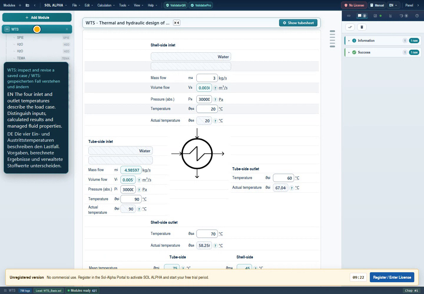
123Unmodified frame from the approved WTS video of 6 September 2026 at 104 s. Shows WTS context, not a newly captured BIL/PSYC/MIFL/JTHO/NETZ mask. Visible notices and display limitations remain unchanged.
- Inside/outside streams in the actual WTS operating context.
- Assign inlet and outlet temperatures to their corresponding sides.
- Shell-side outlet: distinguish target and rated temperature before transferring data.
TIME addresses time-dependent heating and cooling. Initial value, stored mass or heat capacity and time-dependent heat transfer or heat input are essential. A steady final temperature does not establish when it is reached. For the simplest idealized uniform body with constant UA and mc, τ = mc/(UA); phase change, large internal gradients or changing surroundings require review of other assumptions.
This time constant provides engineering orientation, not a claim to describe TIME's complete algorithm. Before use, review the actual module variant, initial conditions, geometry and permissible simplifications. Adding a time value to a previously steady WTS or NETZ case does not create a defensible transient model.
Back to top ↑Chapter 20Find balance errors and conflicting states
| Observation | Targeted check |
|---|---|
| Both BIL duties have the same sign | Compare inside/outside, inlet/outlet and loss term with the source equation. |
| Duty agrees but area does not | Check ΔT pairing, duplicate FN correction, k area basis and actual/required area. |
| Temperature does not respond to a change | The sought value may be prescribed, linked or not yet recalculated. |
| Humidity differs by a factor of 100 | Check percentage display against dimensionless fraction. |
| Mixed enthalpy flow is wrong | Weight J/kg dry with dry-air flow; distinguish total mass. |
| Density disagrees with 1/v | Check dry-air basis: ρmoist = (1+x)/v. |
| JTHO result appears to have the wrong direction | Check upstream/downstream fields and which temperature was actually prescribed. |
| Two-phase message | Respect the model limit; do not transfer it as a valid gas state. |
| NETZ converges but result is implausible | Check topology, exchanger pairing, boundaries and overall energy. |
| Saved curve gives unexpected values | Compare composition, pressure, units, revision and interpolation range. |
Start with the first quantity that disagrees with the task description. Explain incorrect composition before correcting enthalpy. Resolve a wrong temperature reference before optimizing area. Arbitrarily fixing several output values can conceal a mistake but supplies no additional physical information.
Compare baseline and changed cases through a few meaningful quantities: mass balance, heat duty, temperature pairs, humidity basis, phase and relevant geometry. Messages, blank values and incomplete calculation states form part of the finding. Do not document a saved old value as a newly calculated result.
For an actual difference between program versions, preserve the smallest reproducible case with sources, module version and input status. This handbook changes no calculation modules; runtime diagnosis is a separate task and must not silently overwrite historical evidence.
Back to top ↑Chapter 21Save, reopen and release results
Save the native case with a clear task description. Include property files or their unambiguous revision, curves, connections, boundaries and the role of important inputs. A report of final values is a useful snapshot but not automatically a complete model archive. Bundled examples.json documents regressions; it is not a directly loadable SOL project.
- Save the calculated baseline and record fluid state, units, input status and sources.
- Create a changed case under its own name. Preserve the reference.
- Reopen an intended copy. Compare prescribed/free quantities, connections and results.
- For NETZ, also compare nodes, links, pairs and inlet boundaries. For KOKU/RKS, compare composition, pressure and curve data.
- Change one small acceptable quantity and restore it. Check both response and return to the reference.
- Hand over the case with applicable model limits and outstanding evidence.
This is a prepared acceptance template. New BIL/PSYC/MIFL/JTHO/NETZ save, connection or reopening runs were not executed for this edition. The historical JTHO inverse case is likewise not evidence of a newly executed forward roundtrip. Original regression files remain unchanged.
Before engineering release, assess the complete task as well as the algebra: balance closure, target temperature, phase, property domain, required area, suitable hydraulics and consistent network boundaries. Economic results additionally require cost revision and assumptions. Successful software status and an accepted engineering case are different statements.
Back to top ↑Chapter 22Look up fields and reference quantities
This selection covers 110 specific identifiers. Multiple values in a row follow the stated order. Module units come from reviewed definitions; display units may differ. Units such as J/kg become unambiguous only with the correct reference mass. This is not an instruction to lock every field as an input simultaneously.
BIL
| Field | Quantity | Module unit | Role and guidance |
|---|---|---|---|
| BIL: V1 / 2 | Inside/outside mass flow | kg/s | Actual process streams with an explicit sign convention. |
| BIL: V3 / 4 / 5 / 6 | Volume flows / densities | m³/s / m³/s / kg/m³ / kg/m³ | V̇ = ṁ/ρ; use the same state basis. |
| BIL: V7 / 8 | Heat capacities | J/(kg·K) | Mean or justified constant values. |
| BIL: V9 / 10 / 11 / 12 | Inside inlet/outlet, outside inlet/outlet | °C | Inside/outside do not automatically mean hot/cold. |
| BIL: V13 / 14 / 15 | Inside/outside duties / loss | W | Source equation V13 + V14 = V15; check signs. |
| BIL: V16 / 17 | Film coefficients | W/(m²·K) | Distinguish from wall conductivity and overall k. |
| BIL: V18 / 19 / 20 | Wall conductivity / thickness / fouling | W/(m·K) / m / m²·K/W | Use compatible geometry and area references. |
| BIL: V21 / 22 / 23 | Required area / LMTD / overall k | m² / K / W/(m²·K) | A = |Q/(k ΔT)| in the reviewed route. |
| BIL: V24 / 25 / 26 | Outside/inside diameter / arrangement | m / m / − | Counter=1, parallel=2, cross=3 in V26. |
| BIL: V29 / 30 | Mean calculation temperatures | °C | Derived quantities locked by the source. |
| BIL: V31 / 32 | Wall temperatures | °C | From the correct heat flow and area reference. |
| BIL: V33 / 34 / 35 / 36 | Latent enthalpies / phase fractions | J/kg / J/kg / − / − | Special route; sensible heat alone is insufficient. |
| BIL: V39 / 40 / 41 | FN factor / inlet pressures | − / Pa / Pa | Retain arrangement and fluid-state references. |
| BIL: V45 / 46 / 47 / 48 | Tube count / length / actual area / margin | − / m / m² / % | Margin is derived; negative margin stays visible. |
PSYC
| Field | Quantity | Module unit | Role and guidance |
|---|---|---|---|
| PSYC: V6 / 7 | Wet-/dry-bulb temperature | °C | Mask-defined reference; the two states are not interchangeable. |
| PSYC: V8 / 9 | Total pressure | Pa | Absolute air pressure; V9 follows V8 in the source route. |
| PSYC: V10 / 11 | Relative humidity | % | V10: saturated reference; V11: actual air state. |
| PSYC: V18 / 19 / 20 / 21 | Saturation/partial pressures | Pa | Partial pressure differs from total pressure. |
| PSYC: V22 / 23 / 24 / 25 | Humidity ratios / saturation humidity ratios | kg/kg | Water per kg dry air. |
| PSYC: V26 / 27 | Degree of saturation | − | x/xs; not numerically identical to relative humidity. |
| PSYC: V28 / 29 | Specific enthalpy | J/kg | Mass basis is dry air. |
| PSYC: V30 / 31 | Specific volume | m³/kg | Volume per kg dry air. |
| PSYC: V32 / 33 | Moist-air density | kg/m³ | (1+x)/v, not simply 1/v. |
MIFL
| Field | Quantity | Module unit | Role and guidance |
|---|---|---|---|
| MIFL: V6 / 7 / 8 | Inlet and mixed temperatures | °C | Together with states and mass flows. |
| MIFL: V12 / 13 / 14 | Total pressures | Pa | Establish mixing location and pressure equalization. |
| MIFL: V15 / 16 / 17 | Relative humidities | % | Do not take their arithmetic mean. |
| MIFL: V24 / 25 / 26 | Humidity ratios | kg/kg | Dry-air basis; distinguish any liquid phase. |
| MIFL: V30 / 31 / 32 | Moist-air mass flows | kg/s | Separate from dry-air mass flows. |
| MIFL: V33 / 34 / 35 | Dry-air mass flows | kg/s | Weights in the enthalpy balance. |
| MIFL: V48 / 49 / 50 | Enthalpies | J/kg | Per kg dry air. |
| MIFL: V54 | Condensed-water flow | kg/s | Steady mass flow, not stored mass in kg. |
| MIFL: V61 / 62 / 63 | Volume flows | m³/s | At the respective local states. |
JTHO
| Field | Quantity | Module unit | Role and guidance |
|---|---|---|---|
| JTHO: V2 / 3 | Upstream/downstream temperatures | °C | Historical case prescribes V3 and solves V2. |
| JTHO: V4 / 5 | Upstream/downstream pressures | Pa | Absolute; source converts internally to bar. |
| JTHO: V6 / 7 / 8 / 9 / 10 / 11 | N2 / CH4 / CO2 / C2H6 / C3H8 / C4H10 | mol-% | Check composition and sum. |
| JTHO: V20 | Natural-gas selection | − | Historical case uses natural gas L = 2. |
| JTHO: V22 / 24 / 25 | H2 / pentane / hexane | mol-% | Do not silently omit additional components. |
ABGV
| Field | Quantity | Module unit | Role and guidance |
|---|---|---|---|
| ABGV: V1 / 2 | Measured CO2/CO fractions | − | Distinguish dry/wet basis and fraction/percent. |
| ABGV: V3 / 4 / 5 | Flue temperature / air humidity / heating value | °C / kg/kg / J/kg | Document state and heating-value bases. |
| ABGV: V10 / 12 | Flue-gas/incomplete-combustion loss | − | Result quantity, not automatically an accepted efficiency. |
| ABGV: V26 | Fuel selection | − | Match actual fuel and data revision. |
NETZ additionally contains graphical node/link data and repeated heat-exchanger groups. These are managed through the actual plan editor; a long list of internal field numbers would not replace topology. See the NETZ chapter for model limits.
Back to top ↑Chapter 2320 common questions about process calculations
What does BIL actually balance?
The reviewed scope is a heat exchanger with inside/outside streams, thermal area and geometry. Its short name does not imply automatic solution of arbitrary reactions or complete plant flowsheets.
Is the inside always the hot stream?
No. Inside/outside describes equipment assignment. Temperature and heat flow determine which side heats or cools. Retain correct side assignment in child modules and results.
Why is a heat duty negative?
With Q̇ = ṁ(hout−hin), cooling a stream is negative. Positive transferred magnitude and signed stream balance are different representations and must be identified.
Can I simply prescribe V15 as a positive loss?
Check source equation V13 + V14 = V15 and the intended physical direction. The word loss alone does not define its algebraic sign. The teaching case uses zero.
When is Q̇ = ṁcpΔT sufficient?
When the selected mean or constant cp suitably represents the state path and no latent heat is omitted. Use appropriate enthalpy differences for strong property changes or phase transitions.
Does balance closure prove sufficient area?
No. Both streams can release and receive the same duty while actual area is below required area. Also assess driving difference, overall k, area and rated states.
What do equal terminal temperature differences mean?
Equal positive terminal differences give a well-defined LMTD limit: the common difference. Direct 0/0 substitution is not evidence that the process is impossible.
Why must FN not be applied twice?
An already corrected temperature difference includes the arrangement effect. Multiplying again reduces the driving difference a second time and changes area without a new physical basis.
Is wet-bulb temperature the dew point?
No. PSYC uses the wetted thermometer of an aspiration psychrometer. Dew point is a different state quantity. Inputs must match the measurement method actually intended.
Are PSYC columns inlet and outlet?
They represent the wet reference and dry-thermometer/air states. V6 and V7 are not interchangeable process locations. The historical example uses 50 °C wet and 60 °C dry.
Are relative humidity and degree of saturation equal?
No. Relative humidity uses a partial-pressure reference; degree of saturation uses x/xs. In the historical PSYC case, about 58.919% relative humidity corresponds to degree of saturation 0.53433.
Why is 1/v not moist-air density?
Specific volume here is per kg dry air. Total moist-air mass also includes water: ρ = (1+x)/v. The kilogram reference is decisive.
Which mass flows weight MIFL enthalpy?
Dry-air flows weight dry-air-based enthalpies. Total moist-air flows require the appropriate conversion first. This distinction remains when humidity changes.
May I average relative humidities?
Not as a general mixing rule. Balance water and energy on a consistent mass basis to obtain the mixed state. Relative humidity also depends on temperature and pressure.
Is MIFL V54 stored water inventory?
The reviewed module unit is kg/s. V54 describes condensed-water flow in a steady model. Collected mass in kg requires time integration and an appropriate separation/accumulation balance.
Why does the JTHO archive show 50.36315 °C?
It is the sought upstream temperature. Downstream temperature is prescribed at 50 °C. This is inverse calculation, not a forward claim that this gas warms during expansion.
Does adiabatic also mean isentropic?
Not generally. A throttle may operate irreversibly without external heat. The JTHO route here is isenthalpic under its assumptions, not an ideal turbine expansion.
Can I continue JTHO after a two-phase message?
The examined source aborts on detected gas/liquid two-phase conditions before or after the throttle. Establish the appropriate phase/process route; do not ignore the message.
Is NETZ the hydraulic RNET module?
No. NETZ handles a steady heat-exchanger/plant network; RNET handles pipe-network hydraulics. Assign data, topology and boundaries to their respective models. The editors are not interchangeable.
What is actually verified in this handbook?
Sources, package membership, historical example data, independent algebra and the static DE/EN interface are checked. New standalone-module, connection, editor and reopening runs are not claimed for this edition.
Back to top ↑Chapter 24Compact glossary and transfer data
| Term | Meaning |
|---|---|
| Steady | No relevant time-dependent accumulation in the considered balance volume. |
| Transient | State and stored mass/energy change with time. |
| Sensible heat | Enthalpy change represented by temperature change in the selected model. |
| Latent heat | Enthalpy contribution of phase change. |
| Enthalpy reference | Defined reference state; retain consistency when combining data. |
| Dry-air basis | Quantity per mass of dry air, with water mass tracked separately. |
| Relative humidity | Water partial pressure/saturation pressure in the stated model. |
| Humidity ratio | Water loading per kg dry air. |
| Degree of saturation | Ratio x/xs, not generally equal to relative humidity. |
| Dew point | Temperature of initial saturation along the appropriate cooling path. |
| Isenthalpic | Specific enthalpy remains constant during the considered state change. |
| Adiabatic | No heat transfer across the specified external boundary. |
| FN correction factor | Temperature-difference correction associated with an arrangement. |
| Design / rating | Find required geometry / evaluate operation of existing geometry. |
| Balance residual | Remaining difference of balanced quantities, with signs and scaling. |
A transfer to the next module usually needs more than value and unit. Also identify substance, composition, phase, pressure reference, mass basis, state location, data revision and calculation direction. Equipment additionally needs geometry and area basis; a network needs topology and boundaries; a curve needs axes and validity domain.
The 15-member package assignment is preserved even though BIL and FN work closely with heat-transfer modules. Cross-links lead to complementary handbooks without changing actual membership. Individual manuals for special variants remain independent of this complete package map.
Back to top ↑Chapter 25Sources, image provenance and reviewed scope
Web revision: main13.0 / 1cd12e8b173ba72aa5c95c98a14772b7ee537997. All-Dev revision: fix-iteration/v10 / 40606b705b2df95e550ffef5e98ab733ccc66229. The source inventory records package membership, registered tasks, examined BIL/PSYC/MIFL/JTHO/ABGV/NETZ definitions, masks and selected calculation routes with SHA-256. File hashes identify the actual reviewed state even when a working tree contains local changes.
The historical example data come from repository regressions PSYC dated 6 May 2026 and JTHO dated 27 June 2026. Inputs, derived defaults, expectations, original paths and hashes remain distinguishable. The JTHO case is inverse, with prescribed outlet temperature. Neither regression was newly executed in SOL during this work. Original plugin build and comprehensive Desktop/Web parity are not independently established.
Primary engineering references
- NBS Report 9818, Algorithms for Psychrometric Calculations: thermometer temperatures, humidity parameters and dry-air-based quantities. This historical reference does not establish identical implementation of every PSYC algorithm.
- DOE Fundamentals Handbook, Heat Transfer, Volume 2: energy flow, heat transfer and log-mean temperature difference.
- NIST: The Joule-Thomson process in cryogenic refrigeration systems: engineering context of throttling. The specific natural-gas composition and calculation direction are established by our own JTHO archive and module source.
Illustration and verification
Both images are unchanged frames from the approved WTS video of 6 September 2026 at 104 and 225 s. Image provenance records original hashes and capture context. Numbering is separate from original pixels. They show actual process data in WTS context, not new standalone masks or NETZ editor acceptance.
Documentation checks cover algebra, source integrity, chapters, links, images, language, search, mobile layout and offline use. They do not certify a calculation engine. New module, connection, curve-import, editor and save/reopen runs remain separate execution evidence to obtain. The 15-member package map is complete; standalone full manuals for every member and variant are not thereby complete. The manifest records scope.
Back to top ↑